TempLS global temp down 0.03°C in July

The TempLS monthly anomaly for July 2013 was 0.469°C, compared with 0.499° in June. This continues a sequences of small changes. Satellite indices decreased more.

Here is the spherical harmonics plot of the temperature distribution:



Warm spots in East US and N Europe. Australia also continued its long warm spell. Arctic rather cool.


And here is the map of stations reporting:

Buffers, pH and ocean acidification

This post is a followup to some recent discussion of ocean acidification at Climate etc, which provoked scorn from Stoat, and in turn snark from WUWT.

Inevitably, the first comments are along the lines of "can't be acidification until pH7" (never with a reference). I blogged on that here. I'd like to take up two points from that - Lewis acidity and buffers. The general aim of this post is to put pH in context. It's over-used.

Lewis Acid

Early definitions of acidity relied on the properties of hydrogen ions, and of course pH is central. But in 1923, Lewis generalised the notion of acidity to the sharing of electron pairs, which needn't involve hydrogen.

That's an important simplification. In fact, H+ has very little final role in the seawater reactions. You can express them as:
CO₂ + CO₃^-- + H₂O ⇌ 2HCO₃^-
Ca⁺⁺ + CO₃^-- ⇌ CaCO₃
No protons, but the Lewis acid CO₂ reacts with the base CO₃^--, shifting the solubility equilibrium.

Buffers

Buffering is often thought of as pH buffering, but again I'll aim to generalise. In fact, it's just a consequence of ternary equilibrium:
H + A ⇌ HA
The Law of Mass Action gives the equilibrium relation:
[H][A]/[HA] = K
If K is of moderate size, and [H] is small relative to [A] and [HA], then whether the reaction moves back or forward, [H] remains relatively fixed because the dominant species don't change much in proportion.

The familiar pH version arises when HA is a weak acid and [A] a weak base. Then [H⁺] is small, and relatively fixed (buffered) by the equilibrium.

A common sceptic scoff at acidification is, how could so few H⁺ ions make a difference? At one level it's right - they can't directly. But what buffering means is that if [H⁺] changes, then something else has changed, by a lot. And that is what is likely to cause changes.

Sea-water reactions

These were listed above:
CO₂ + CO₃^-- + H₂O ⇌ 2HCO₃^-
Ca⁺⁺ + CO₃^-- ⇌ CaCO_3(aragonite)
I'll ignore the effects of hydration of both H⁺ and CO₂

There is an excellent review article by Zeebe which sets this out in much more detail, and I'll refer to it later.

The effect is that when CO₂ is added, the first equilibrium shifts to the right, CO₃^-- is diminished, shifting the second equilibrium to the left. The equations can be combined:
CO₂ + CaCO₃ + H₂O ⇌ 2HCO₃^- + Ca⁺⁺
This emphasises that ultimately each extra molecule of CO₂ tends to dissolve a molecule of CaCO₃, if equilibrium shifts to the right.

pH Equilibrium relations

The equilibria can also be expressed as the more traditional diprotic acid-base expressions

CO₂ + H₂O ⇌ HCO₃^-+ + H⁺; pKa=5.94

HCO₃^- ⇌ CO₃^--+ + H⁺: pKa=9.13
The pKa values are the log10 of the equilibrium constants.
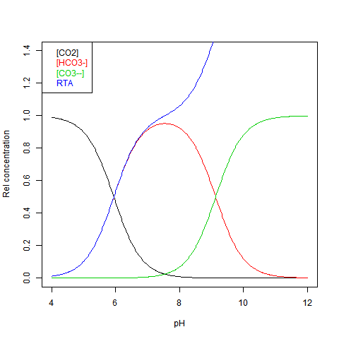
The equilibrium can be shown against pH as Bjerrum plot. This shows relative concentrations normalised against DIC = dissolved inorganic carbon. This is just the sum:
DIC=[CO₂]+[HCO₃^-]+[CO₃^--] Here is the plot:

RTA stands for Relative (to DIC) Total Alkalinity - see next.

Equilibrium relations - some numbers

I'm following the Zeebe review article here. Typical values for dissolved species:

• DIC 2.05E-3 M (M = 1 mol/l ~ mol/kg)
  
• Total Alkalinity=[HCO₃^-]+2*[CO₃^--] = 2.35E-3 M
  
• ratio %: [CO₂]:[HCO₃^-]"[CO₃^--]=0.5:89:10.5 at pH 8.2
  
• So [CO₂]=1E-5 M, [HCO₃^-]=1.82E-3 M, [CO₃^--]=2.1E-4 M
  
• At pH 8,2, [H⁺]=6.3E-9 M; [OH^-]=1.6E-6 M;
  

Sea Water measurement

Eli had a post arising from these threads on pH measurement. It's hard. However, there is a new method, probably less accurate, but suitable for continuous monitoring. It uses an ion-selective field FET, SeaFET, which can be set in place for months at a time. But, as insisted here, pH is over-emphasised. It follows the major species, and they can be used to measure it. Two quantities easily measured by flask analysis are all you need. One is DIC. This can be measured gravimetrically. The other is Total Alkalinity (TA) TA=HCO₃^-]+2*[CO₃^--] This can be determined by acid titration with an indicator that changes about pH=4.5, which removes almost all bicarb and carb. The titration also picks up borate and hydroxide, and [H+] needs to be subtracted, but these are small effects which I will ignore here. All you need are the values of DIC and TA - both easily obtained by flask analysis. The point is they are present in much larger concentrations, and are more stable.

Use of equilibrium relations

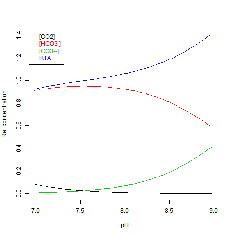
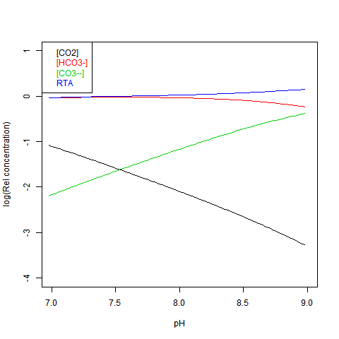
Given DIC for normalisation and any other concentration (in particular TA), you can read a pH value from the Bjerrum plot, and deduce everything else. But here are some more convenient log plots. Firstly with pH again on the x-axis, but log10 on the y-axis. Note that both log([CO₃^--]) and log([CO₂]) vary close to linearly
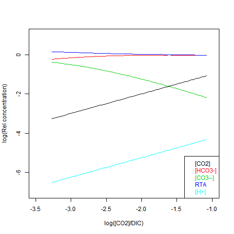
Now shifting the relative total alkalinity RTA to the x-axis. This allows the other values to be read explicitly:
 
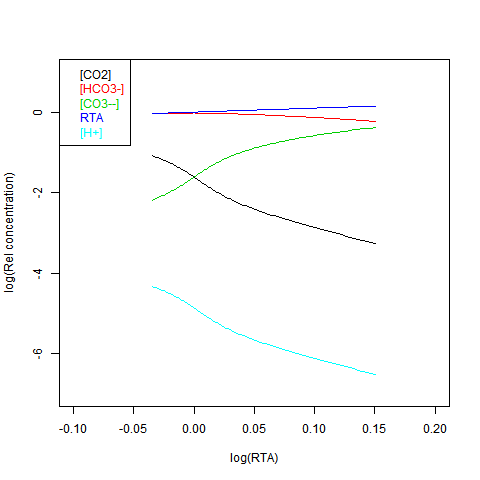
RTA is easily obtained, but doesn't preserve the linear relations. Here is log([CO₂]) on the x-axis:

Solubility equilibrium

The end problem is dissolution of CaCO₃ structures. Two reasons are sometimes given why this may not matter

• 
  Biological deposition is complex - not just a solubility product
  
• The oceans are supersaturated relative to aragonite formation (the CaCO₃ form used by most organisms).
  

Deposition is complex, though I have trouble believing that reducing [CO₃^--] won't make it harder. But in any case, the structure once formed has to resist solution, at all times, when conditions are fluctuating. Another reason advanced for unconcern is that pH continuously monitored shows fluctuations large relative to the long term changes wrought by CO₂ increase. It's not clear whether these track changes in carbonate, but if they do, then clearly the structures are intermittently exposed to dissolving conditions much worse than average. And dissolving once is enough.

Discussion

What I hope these plots will show is that pH is just one of a number of co-varying quantities, and because of the small number of ions represented, is far from the most important. You can use it to track the reaction if convenient, but you don't have to. It's an intermediate - the nett reaction is CO₂ neutralising CO₃^--, producing HCO₃^-. This then affects the CaCO₃ solubility equilibrium. The secondary role of pH is relevant to the following things that have been said in the acidification discussions:

• "Acidification requires pH<7
  pH is just an indicator of the carbonates equilibrium. pH 7 has no relevance.
  
• The number of H⁺, even with acidification, is too small to matter
  True, H⁺ are not the problem
  
• pH measurements are sparse and inaccurate
  But not TA/DIC, which is enough.
  

June GISS Temp up by 0.12°C

GISS LOTI went from 0.55°C in May to 0.67°C in June. Since TempLS rose by only a small amount, this is an unusually large discrepancy. Satellite lower troposphere temperatures also rose by even greater amounts.


Here is the GISS map for June 2013:



And here, with the same scale and color scheme, is the earlier TempLS map for June:

Previous Months

May
April
March
February
January
December 2012
November
October
September
August
July
June
May
April
March
February
January
December 2011
November
October
September
August 2011

More data and plots

TempLS global temp up 0.02°C in June

The TempLS monthly anomaly for June 2013 was 0.498°C, compared with 0.48° in May. Satellite indices rose by about 0.2°C, but from a low base.

Here is the spherical harmonics plot of the temperature distribution:



The pattern is oddly similar to last month, with a cold spot in central Asia and warmth each side, and W Europe and India cold. But the Alaska warmth shows up.


And here is the map of stations reporting:

A climate blog index

In an earlier post I described my dabblings in RSS files trying to get a replacement for Google Reader, now passé. As a by-product, I posted a climate reader.

I've improved this, mainly by rationalizing the way it uses the RSS info. It's easier to extend to more complex formats, and more concise, so quicker to download. The new version is below the jump, with instructions following. I'm now inclined to call it an index, because that is what it is good at. You can't read content directly, only by link to the blog. That may change, but the limit is on how much can be downloaded.

Mainly, you can order by topic, blog, date or commenter, and you can subset on any of those. I'll make this version a page, which will be the maintained version. Some time soon, I'll have to include a paging version.
Update - the paging system is done. Top right there is a month selector, with Add/Set. Select a month, and either add it to the data shown, or replace that data (set). By default, the current month and last full month are shown.







It shows all the posts and comments that it is aware of. Updating is hourly. You can click the buttons at the top to reorder. Main posts are indicated by a background color.

You can select subsets. You'll see four selection boxes top right. If they are empty, everything passes. Otherwise, for three of them, you can enter names, and only those will show. You can select commenters, blogs and threads. Time is different. You can select one or two times. If one, it will show only posts more recent. If two, it will show posts between those dates.

On the right you'll see a selection panel. The steps are:

1. Click on one of the selection boxes on left. It will turn pink to show it is active.
   
Make a name appear in the Result section on right (see below for how)
2. Click Enter. Your selection will be at the bottom of the list.
3. You can click delete to remove the top item in the active list.

There are two ways to enter a result. The simplest is to find a line displayed that has the aspect you want. Then click at that level on the red bar that is to the right of the table. You may have to click twice. Your selection should appear. If it is what you want, press enter.

The second way is to enter the first few letters in the text box, top right, and then click. If it gets something else, add more letters. Again, when it is right, press enter.

To make your selection show, just click one of the four column buttons, depending on the ordering you want.

Issues

Some blogs don't easily pass comment information. Planet 3 is itself an aggregator, so I haven't really cracked that. As I mentioned in the previous post, SkS doesn't give comment dates, so I can't tell what is new in each RSS read - I haven't solved that yet.

Better adjusted global temperatures for ENSO, Solar and volcanoes

This is a follow-up to this earlier post, which please see for details. I had got into some difficulty there with using the R function nlm() to estimate both the regression parameters and the delay coefficients for each of the exogenous variables Vol, Sol and ENSO. The solar variable, which interacts most weakly, was apt to be assigned zero or negative delay, which created constant or exponentially rising secular processes, which were used by the fit.

I could avoid this by constraining that parameter. But I think it is better to do as others have done and use a common delay for all three. There is reasonable physical justification for that, and it reduces overfitting.

The result is a much more stable trend pattern across the time intervals and data sets. The trends since 1997 are now mostly between 0.65 °C/century and 1.325. This might still be seen as a slowdown, but surely a minor one. Oddly the only exception is the case studied by SteveF, Hadcrut 4 with linear from 1950. The trend I got there was 0.117°C/cen, I think quite similar to his, as was the decay coefficient at 0.026 (cf his 0.031).

I'll show below the revised table and images.

A zip file of R code and data is here.

Results

Here is the table. The results look better in several ways:

• The coefficients are reasonably comparable across cases
• Adding a quadratic term now always reduces the sum of squares
• The post-1997 trends are fairly uniform

I have not normalised the units, so the actual magnnitudes of the regression coefficients are not easy to interpret. I'd still discount the 1979 quadratic, although no problems are obvious.

	Start	Trend	1	Vol	Sol	ENSO	t	t^2	Delay	SS
HADCRUT4	1950	0.117	2e-04	-8.39135	-3e-05	0.42995	0.25141	NA	0.02584	10.079
HADCRUT4	1950	1.024	-0.07304	-2.27873	0.00048	0.14844	0.30742	0.21653	0.12729	8.254
HADCRUT4	1979	1.086	-0.01689	-2.72106	0.00069	0.13331	0.50485	NA	0.11706	3.909
HADCRUT4	1979	1.078	-0.00963	-2.82278	0.00069	0.13478	0.50155	-0.07812	0.11325	3.893
GISS	1950	0.787	-0.00116	-6.00112	5e-05	0.24419	0.34476	NA	0.04173	10.441
GISS	1950	1.246	-0.04836	-2.70426	0.00042	0.1288	0.37122	0.14273	0.11017	9.626
GISS	1979	1.325	-0.01623	-3.28644	0.00065	0.1334	0.49335	NA	0.09649	5.086
GISS	1979	1.315	-0.01142	-3.38601	0.00064	0.13513	0.48994	-0.05241	0.09342	5.079
NOAA	1950	0.65	-0.00121	-4.42051	0.00017	0.19036	0.33218	NA	0.06223	8.103
NOAA	1950	0.877	-0.04486	-2.39086	0.00042	0.13126	0.34807	0.13221	0.118	7.351
NOAA	1979	0.929	-0.01586	-2.81475	0.00059	0.12721	0.47137	NA	0.10492	3.581
NOAA	1979	0.913	-0.00629	-2.99252	0.00058	0.13034	0.46551	-0.10409	0.09849	3.554

Images

The images may be scanned in the viewer below. There are 24, and you can flip through them using the top buttons. But you can also subselect using the selection boxes. For example, if you choose GISS, you will then cycle through just the 8 GISS plots. If you ask as well for plot type components, you will cycle through the four component plots. etc.

Data All Hadcrut 4 GISS NOAA Start Year All 1950 1979 Regressor All Linear Quadratic Plot type All Temp Series Components

SteveF has had difficulty getting comments through the system - I'm trying to find out why. Anyway, he sent by email these comments, and I'll just follow with a few points I made in reply - hope we can get comments working for him soon:

SteveF says:

I think I may have identified why the influence of the solar cycle increases in the 1979 to present analyses compared to the 1950 to present analyses: there is a coincidental congruence between the 1983 and 1991 volcanoes and the peak (or near peak) of the solar cycle. That is, the downward part of the solar cycle is aliased with the volcanic influence. In the longer series, this influence is diluted in the regression, though for certain is still influencing the results. The 1964 to 1970 eruptions, while weaker, do not coincide with the peak of the solar cycle. I have tried several things to straighten this out, so far without a lot of success. I will next try a regression from 1950 to 1975 to see if the solar cycle influence falls to almost nothing (or even negative!) as I suspect it will. Substituting a regression specified quadratic or cubic secular function.

I think a defensible argument is, absent a good physical rational, that the best approach is to simply sum the two radiative terms (both with watts/M^2 units) and see what happens to the diagnosed "optimal lag". Any regression that reports a physically implausible lag constant for best fit seems to me very suspect. There have been multiple published reports with estimated lags for volcanoes; a tau value near 30-36 months for the decay of the response seems to be a common, though the exact value depends weakly on assumed climate sensitivity value (I have independently verified this is correct). Perhaps the best thing is to just try a few lags in the credible range and see what the best fit regression constants turn out to be. I also note that very much higher solar than volcanic response (on a watt/M^2 basis) is exactly the opposite of what I would expect on physical grounds; the slower solar cycle response ought to be lower, on a degrees/watt/M^2 basis than the volcanic, because the 11 year solar cycle 'sees' slower responding (deeper) parts of the oceans more than the shorter volcanic forcing. 

If one accepts a large discrepancy between the measured changes in solar intensity over the cycle and the size of the temperature response, then some kind of 'amplification' of the solar cycle must be responsible (eg. more low clouds at the minimum), and evidence for that seems lacking. Of course, even if one assumes the true solar cycle forcing (in watts/M^2) is far higher than the measured changes in solar intensity, that doesn't mean there should not be considerable lag in the temperature response.

Finally, I tried a linear secular trend starting in 1964 (to include the earlier volcanoes); the fit is improved compared to starting in 1950 and the discrepancies between model and Hadley global temperatures is much reduced. Perhaps you could try that as well.
Nick says: I can well imagine that solar cycles might get tangled with volcanoes. My experience was the the solar cycle, being weak, could be pushed around a lot by the optimisation process - both the linear and the lag fitting. It had a strong tendency to drift into zero or negative lag, which nlm() took advantage of to create spurious fitting functions. For the same reasons, I don't take too much notice of the amplitude that emerges from regression. It could be just taking up a bit of the volcano signal.

My main concern at the moment is with the use of Nina34. I think it's a sensitive index, but also includes warming trend, and when you adjust with it, it takes out that part. I'm inclined now to switch to SOI, which may not be as good, but can't drift. A practical alternative is to detrend Nina34, but harder to justify, and the detrend would depend on the interval. I'd be happy to try a 1964 start. Another option is to use GHG forcing as one of the regressor functions.

May GISS Temp up by 0.05°C

GISS LOTI went from 0.51°C in April to 0.56°C in May, almost exactly matching the rise shown by TempLS. Satellite measures went down slightly.




Here is the GISS map for May 2013:

And here, with the same scale and color scheme, is the earlier TempLS map for May:

Previous Months

April
March
February
January
December 2012
November
October
September
August
July
June
May
April
March
February
January
December 2011
November
October
September
August 2011

More data and plots