Moyhu data updates

For a while now, I have been maintaining updated data tables and graphics. Many are collected in the latest data page, but there are also the trend viewer, GHCN stations monthly map, and the hi-res NOAA SST (with updated movies). These mostly just grew, with a patchwork of daily and weekly updates.

I'm now trying to be more systematic, and to test for new data every hour. My scheme downloads only if there is new data, and consumes few resources otherwise. My hope is that all data will be processed and visible within an hour of its appearance.

I have upgraded the log at the bottom of the latest data page. This is supposed to record new data on arrival, with some diagnostics. Column 1 is date, which is actually the date listed at origin, translated to Melbourne time. The column headed "Delay" is the difference between this date and the date when processing is finished and the result should be on the website. I'm using this to find bugs. The date in the first column isn't totally reliable; it is the outcome of various systems, and may predate the actual availability of the data on the web. The second column is the name with link to the actual data. For the bigger files (size, col 3) a dialog box will ask whether to download. The "Time taken" is the time used by my computer in processing (again, for my diagnostics). Where several datasets are processed in the same hourly batch, this time is written against each of them. Currently, only the top few most recent lines of the log are useful, but new data should be correctly recorded in future.

NOAA temperature is a special case. It doesn't have the files I use in a NOAA ftp directory, but serves them with the current time attached. I have to use roundabout methods to decide whether they are new and need to be downloaded (I use their RSS file). By default they show as new every hour - I have measures to correct this, but they may not be perfect. Anyway, the times in the log for NOAA are not meaningful.

I have a scheme for doing the hourly listening only when an update is likely (assuming approx periodicity). If data arrives unexpectedly, it will be caught in a nightly processing.

It is still a bit experimental - I can't conveniently test some aspects other than just waiting for new (monthly) data to appear and be processed. But I think the basics are working.

Record warm periods

In the previous post, I cited the NOAA June temperatures report. This noted various periods of time with average temperatures that exceeded anything comparable in the record, particularly recent twelve month periods.

Sou has been tracking the average so far in this calendar year. Steve Bloom doesn't like non-physical calendar periods, and prefers the running average. I think Sou's analysis makes sense. It is the best guide to the 2015 year average, since it uses data from that year only. One could say people shouldn't focus on arbitrary year divisions, but they do.

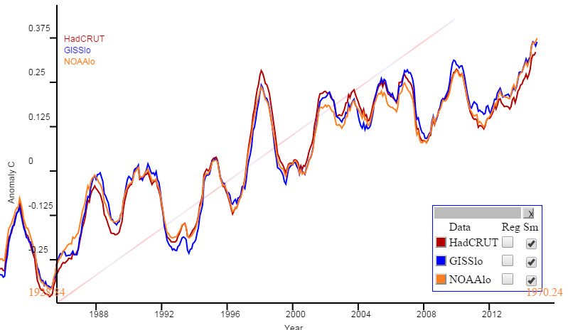
However, if you want running twelve month averages, they are available at the maintained active plot. Just click the buttons on the side table headed Sm. twelve month running is the default (and only) smooth. Here is an example:



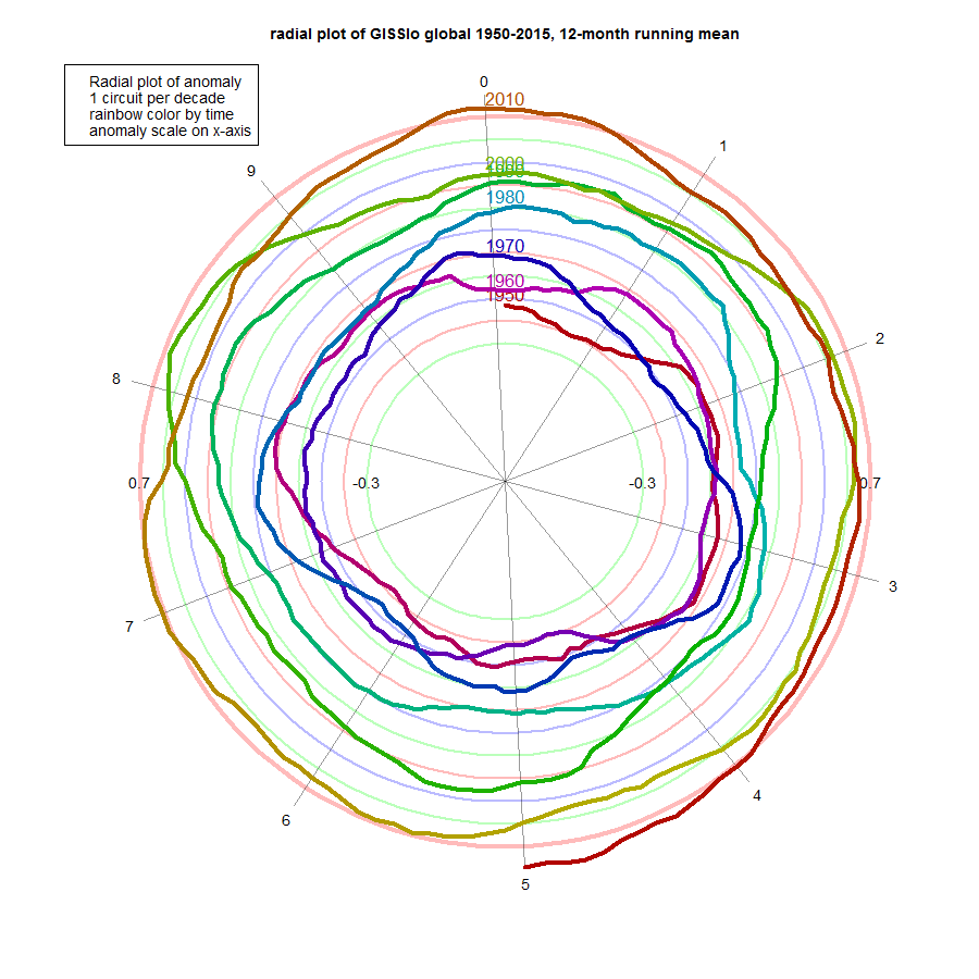
However, in this context, I'm a fan of polar, or radial, plots. Here curves track like a clock with time, with radial distance indicating temperature or other plot variable. I use it for ice extent here. Then there is a natural period of a year, but that isn't essential. The point is that by rolling it up, a long stretch of time can be covered with good resolution (but crowding).

So below the fold I'll show radial plots (with decade winding period) for the main surface indices, from 1950 to now. They will show clearly how warming has continued, as the curve spirals outward, even during the "hiatus". Now they are at record radius, and that is very likely to increase, at least for a little while. The reason is that the change in moving average depends on both the new readings, and the old readings that they replace. Mid-2014 was a relatively cool period, so as long as 2015 is warmer, the running mean will increase.

In these plots, there is a continuous curve in rainbow colors, violet in 1950, and ending with red now. It goes clockwise, 36°/year, crossing the y axis every decade as marked. Radial distance represents temperature anomaly (according to the source) as marked on the x axis, and shown with faint circles. The running mean is centered, so the latest at the bottom shows as Dec 2014.

So here is the NOAA Land/Ocean plot. A curiosity here is that the NOAA report says the maximum 12-month average is 0.83°C; I get 0.81, on their data. But the pattern is the same. Spiralling outward indicates warming, and it is clearly happening, with minor variations, since about the third circuit (70's). And it is now at record level (and has been for six months), and heading outward.



Here is GISS Land/Ocean, which looks much the same:



And here is HADCRUT 4. It probably shows the least adherence to uniform growth, and has more pronounced excursions in 1998, 2005, 2007 and 2010. It's still well in front now, though.



2015 will be a record year if the curve stays outside to previous levels for six more months. And as I said above, a month or two more of expansion is very likely, just on the basis of cooler mid-year 2014.

ps Arctic ice had been holding up fairly well. But it is showing signs of downturn in the last five days, dropping below 2010, and close to 2014.

NOAA up 0.02°C in June; GISS now up 0.04°C

I don't normally post separately for the NOAA NCEI global temperature anomaly index, but this month is the first where everyone is using the new V4 ERSST. There is also a revision of GISS post-V4 (thanks to GISS for the acknowledgement). So it is an opportunity too to review how well TempLS matches in the new environment.

The NOAA report has June at 0.88°C relative to 20Cen; up from 0.86°C in May. GISS is now 0.8°C, up from 0.76°C. Both these are the hottest June in the respective records, and would be close to the hottest month ever, if it were not for Feb-Mar of this year. I have described in my GISS post where it was hot and cold, with more quantitative information here; the NOAA report presents a similar account in more detail.

I have noted earlier how, as expected, TempLS mesh and GISS tend to go together, being interpolated, and NOAA and TempLS grid also have an affinity. Indeed, at times, TempLS and NOAA have been eerily close. With V4 that has been somewhat interrupted, although the general pattern still holds, and the correspondence is currently close. I'll show plots below the fold.

Incidentally, the revised GISS now shows nothing unexpected in the plot of recent monthly differences (earlier version here). Here how it looks now:



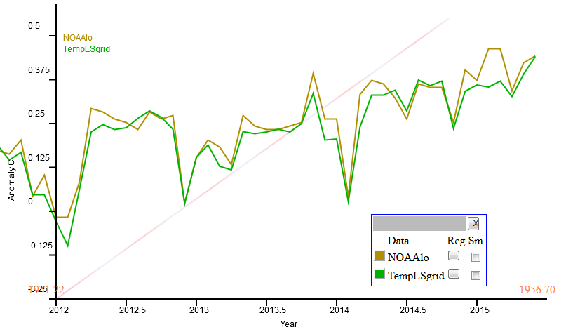
So here is the plot over 4 years of NOAA vs TempLS grid. The plots are made using this gadget, and are set to a common anomaly base of 1981-2010. The divergence earlier this year is the largest. Otherwise the correspondence is good.



And here is the comparison of TempLS mesh with GISS. I think the correspondence is better than before the ERSST change.



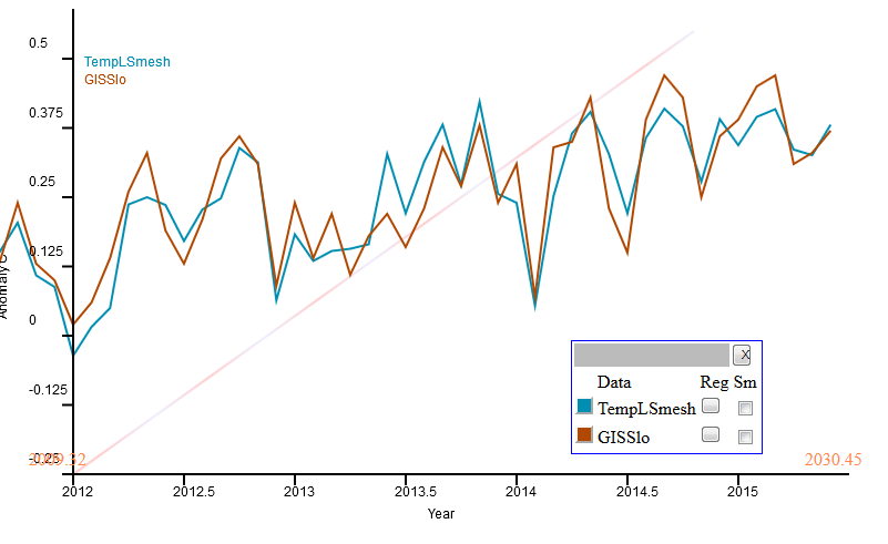
And here is the combined plot. I've used reddish for grid, bluish for interpolated. You can see the pairing, although they are all fairly close. The pairs come together at the end; this is just how it happened.

A breakdown of monthly temperature variation

A by-product of the new TempLS mesh is the analysis that can be done using the arrays of residuals and weights. The weights are mesh areas assigned to stations, and the global anomaly is the thus-weighted sum of residuals. This sum can be partitioned into regions. Two calculations are then of interest:
AveT = sum_R(w*r)/sum_R(w)
which is the average T for region R, and
Contrib_r = sum_R(w*r)/sum_G(w)
which is the proportional contribution R makes to the global T. That means you can see how those contributions add. So instead of saying it was cold in N America, you can see just how much that cold pulled down the global average.

Below the fold I'll show both of those for continent-sized regions, and also the ocean, for the months of 2015. Note that they are not exactly sums over the continent areas, but over the areas that are assigned to nodes within the regions. Each month has a different mesh, so these area assignations vary slightly - I'll show a third plot to quantify that. Of course, the regions don't change (except for ocean freezing), so to the extent it otherwise varies, it's an error.

I'll show how you can see what exactly contributed to the ups and downs of temperature this year.

The regions are Afr=Africa, Asia (without Siberia), Sib=Siberia (Asiatic Russia, code 222), S America, N America, AusNZ=Oceania, Europe, Ant=Antarctica, Arc=Arctic>65°N, Sea=SST, and All=Global. I follow the classification of the GHCN country codes, for which 100-199 is Africa etc. Arctic stations are removed from N Am and Sib.

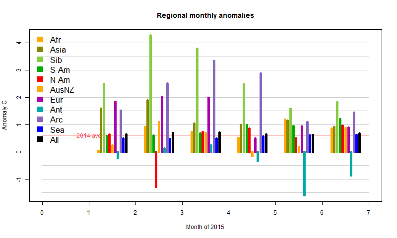
Here is the plot of monthly regional averages. Land regions are very variable compared to Sea and Global. But they are mostly minor components of the sum, and the next plot will show that in perspective. Features are the famous N American cold of February, recent cold in Antarctica, and Feb/Mar warmth in Asia/Siberia. You can also see the Arctic warmth in March/April, which led to early melting.



Now here is the version weighted as contributions to the main sum, which is more informative. The black is the sum of the colors.



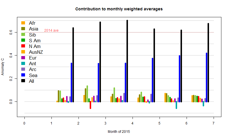
Firstly, SST has been gradually increasing, which pushes the total up significantly, without showing month-month fluctuations. Then you see the sharp cold spell in February N America. It has a small reducing effect, almost countered by a rise in Africa, and dwarfed by the warmth in Asia and Siberia. Consequently, Feb globally was a lot warmer than Jan, despite that cold much remarked on blogs. In May/Jun and even Apr, the cold in Antarctica had an effect, which, with the subsiding warmth in Asia/Siberia, is responsible for later cooling.

Finally, I'll show the variation in weights. There isn't much; I've shown 10x bars faintly over the land regions to make the effect more visible.



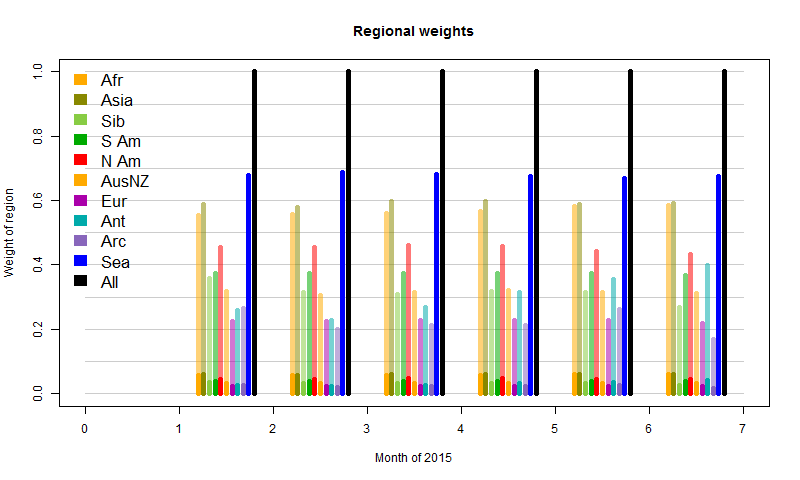
The exception is Antarctica, where the sea ice has been growing. Since that is then excluded from the SST component, land stations carry greater weight as the ocean recedes. The Arctic behaves irregularly. This reflects the fact that the mesh there is sparse, and has a degree of randomness in its response. It reflects the limits of this measure. Still, it's a minor effect overall.

I'll probably incorporate this analysis in the ongoing latest data.

GISS (new version) up by 0.03°C in June

The anomaly for GISS in June was 0.76°C (h/t JCH). This was just as I had expected, since TempLS mesh rose from 0.618°C to (now) 0.673°C. However, meanwhile the GISS May number increased from 0.71°C to 0.73°C, so the rise was not quite as great.

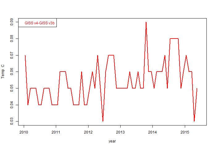
Behind that lies a story. As Olof noted, GISS this month switched from using ERSST V3b to ERSST v4 (I switched last month). They show some plots of the differences here. Here is the difference plot



In the new file April 2015 is the same as before, and May only increased by 0.02°C. But the plot shows an annual difference of more than 0.05°C in recent years. I plotted the monthly differences (GISS v4 - 3b) over the last five years:



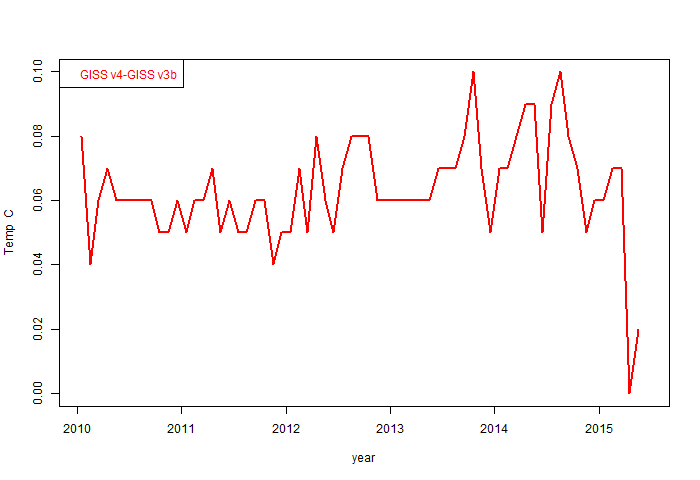
April and May do look quite different. I wonder if GISS is still using v3b there? Anyway, the usual maps and commentary are below the fold:

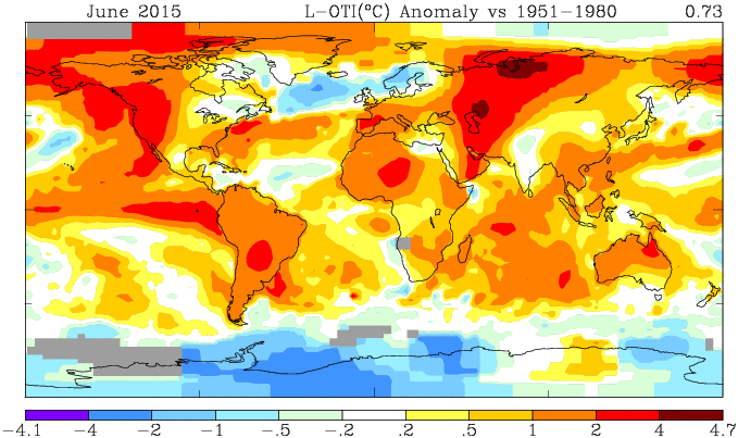
Here is the GISS map for June 2015:


And here is the corresponding TempLS mesh map, based on spherical harmonics:




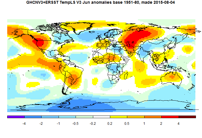
TempLS is somewhat smoothed so doesn't show the peaks of GISS. But the features are just the same. Heat in central and W Russia, and in NW N America. Cool in Antarctica, and N Atlantic, extending over Scandinavia.

You may have noticed that an error had got into my TempLS map plots recently. They were shown with mean subtracted, and so much colder. This has been fixed.

TempLS shows June anomaly up by 0.05°C

Most of the GHCN V3 data is now in, and ERSST v4, and TempLS mesh (the new V3)  shows a rise from 0.618 to 0.665°C, relative to a 1961-90 base period. TempLS grid rose from 0.674 to 0.711 °C. Usually the mesh weighted version is more likely to agree with GISS and the grid version with NOAA, though this time they both are similar.

The rise is somewhat at variance with the NCEP/NCAR index, which suggested a fairly cool month, although that is muddied somewhat by the May oddity when that index suggested more warming than TempLS mesh and GISS showed. Anyway the TempLS calc is certainly warm, and for TempLS grid, seems to be almost a record, falling just short of the 0.718°C for Feb 1998.

The warm places were western US and central Russia, with cold in Antarctica and the E Mediterranean, pretty much as indicated in the NCEP/NCAR report. As I mentioned in my previous post, you can get more detail in the regular WebGL map here, which shows the actual station anomalies with shading between.

There was a curious delay with the Canada data which slightly set back this report. The initial posted data was a duplicate (mostly) of May, and flagged as such, so TempLS rejected it. That seems to have been corrected, and now 4266 stations (incl SST cells) have reported, which is almost all that we can expect.

In other news, Arctic ice has held up well in the last month, but the last two days of JAXA show rising melt, and Neven says more heat is on the way.

Maintained WebGL map of past GHCN/SST station anomaliess

I have a maintained page here which shows anomalies for individual land stations and SST cells, averaged over each month. Land data comes from GHCN V3 unadjusted, and SST from ERSST, formerly ver 3b. It is a shaded color map, with true color for each station, and linear interpolated color in between. I think it's the best way of seeing the raw data.

Now that I am doing daily runs of TempLS mesh, and this produces much of the necessary data, I have decided to make production of these maps a subsidiary process. This saves duplication, and keeps up to date with versions (using now ERSST 4). But what may be more useful is the daily updating. That means that the latest month can be tracked progressively as data comes in. So today, I am waiting on data from Canada and some Latin American countries before posting the TempLS result for June. But you can see it here, and it shows how TempLS calculates its interim result with interpolation. Of course, you could wait till tomorrow when Canada will probably be in.

I have also extended the range back to 1900. You can examine any month in detail. I haven't yet done the annual and decade averages back beyond 1990, but soon.

NCEP/NCAR in June

Data for the Moyhu NCEP/NCAR index is now in. It was a month of contrasts - starting very warm, then cold, and ending somewhat warmer. The end result of 0.204°C (1994-2013 base) puts it similar to January. You can now see the map of average temperatures for the month. Warm in west N America and NE Pacific (strong El Nino pattern), also in W Europe and W/central Russia. Extremes in Antarctica, mostly cold. Cool in E Mediterranean.

As noted here, there is predictable month-month variation associated with choice of anomaly base period. That was partly responsible for the discrepancy between a May rise in the index, and a flat GISS. To try to counter this variation, I have added a section of the table below the monthly indices which tries to put the index on the same anomaly base as GISS or NOAA. It can't do this directly (lacks good data), but can work out that component of the change based on other indices during 1994-2013. IOW, it's the corrected prior estimate for those indices. That estimate is that GISS should be about the same as May (0.72°C), while NOAA should be about the same as April. However, NOAA has been consistently exceeding expectations lately.

Update. Troposphere data: RSS is up from 0.31 to 0.391°C; UAH v6 is up from 0.27 to 0.31.

TempLS V3 - part 3 - results

This is third in a series (part 1, part 2), about TempLS ver 3. The first part gathered a big array x of temperatures of land and sea. The second made an array w (with similar form) of weights, and a combined station inventory iv. As explained here, that is all you need for a simple iterative process to compute temperature anomalies and their average by a least squares process. The code to do that will be described here.

As earlier, we have a control word (job), and the fourth character could be either O,o,P or p. Lower case means skip the stage, so the first line tests this. The rest of the control tells which stored (x,w,iv) to load. Then to make linear ops work, the NA's are removed from x - they can have any value since w=0 there. x and w are re-dimensioned.

if(do[4]){
 load(R[3]) # x are anomalies, w weights
 x[is.na(x)]=0
 d=c(nrow(x),12,ncol(x)%/%12) # stations, months,years
 dim(w)=dim(x)=d 

The iteration proceeds by alternately calculating L, the offsets for each station as the weighted average of temperatures minus G, the global anomaly, and then G as the average anomaly relative to those offsets. These are the calculations that matter; for the rest, changes in G are tested for convergence. Typically each iterations takes a second or two, and six or so may be needed. Note that a tiny number is added to the weight denominators wr and wc for the rare cases where these are zero, leading to a 0/0, which should resolve to 0.

 L=G=v=0;
 wr=rowSums(w,dims=2)+1e-20; wc=colSums(w)+1e-20; # right hand side
 for(i in 1:20){ # gauss-seidel iterations
  g=G
  L=rowSums(w*(x-rep(G,each=d[1])),dims=2)/wr  # Solve for L
  G=colSums(w*(x-rep(L,d[3])))/wc # then G
  if(mean(abs(G-g))<0.0001)break
 }
 if(i>19) stop("Not Converged")

For the rest, there is just post-processing, which you can adapt to your requirements. In the main stream, I just print and store results. The first statement is important, though. There are 12 loose degrees of freedom to add numbers to G by month, and subtract same from L. The calculation gets reasonable results here, but with small arbitrary shifts from month to month. The subtraction fixes these to be right for some fixed time period - typically a 3 decade stretch like 1961-90 here.

For the rest, it's saving output. I have the graphics code (used if the control (job) was "P") on a separate file which I won't plod through here.

# post processing
 G=round(G-rowMeans(G[,62:91]),3)  # Set to basis 1961:90
 ow=c(colSums(w,dims=1)>0) # !ow means no data that month
 G[!ow]=NA  # usually months without data in last year.
 save(G,L,r,w,iv,file=R[4])
 ym=round(outer(0:11/12,yrs,"+"),2)[ow] # months in year units
 write(paste(ym,G[ow]),file="templs.txt")
 if(kind[4]=="p")source("LSpic.r") # graphics
}

So finally, here is the complete code

# Function TempLS3.r. Written in four stages, it collects data, makes weights 
#and solves for global temperature anomaly. 
#Written by Nick Stokes, June 24 2015. 
#See  https://moyhu.blogspot.com.au/2015/06/templs-new-v3.html

isin=function(v,lim){v>=lim[1] & v<=lim[2]}
mth=function(yr){round(seq(yr[1]+0.04,yr[2]+1,by=1/12),3)}
sp=function(s)(unlist(strsplit(s,"")))
pc=function(...,s=""){paste(...,sep=s,collapse=s)}
if(!exists("job"))job="UEGO"
i=sp(job)
kind=tolower(i)
do=i!=kind
yr=c(1900,2015); yrs=yr[1]:yr[2]; # you can change these
ny=diff(yr)+1
j=c(1,1,2,2,1,3,1,4); R=1:4; #R will be the names of storage files
for(i in 1:4){ # make .sav file names
 R[i]=pc(c(kind[j[i*2-1]:j[i*2]],".sav"))
 if(!file.exists(R[i]))do[i]=TRUE; # if filename will be needed, calc
}
if(do[1]){  # Stage 1 - read land (GHCN)
 getghcn=function(){ # download and untar GHCN
  fi="ghcnm.tavg.latest.qcu.tar.gz"
  fi=sub("u",ki,fi)  # switch to adjusted
  download.file(pc("https://www1.ncdc.noaa.gov/pub/data/ghcn/v3/",fi),fi);
  gunzip(fi,"ghcnv3.tar",overwrite=T);
  untar("ghcnv3.tar",exdir=".");
  di=dir(".",recursive=T)
  h=grep(pc("qc",ki),di,val=T) # find the qcu files un subdir
  h=grep("v3",h,val=T) # find the qcu files un subdir
  file.rename(h,Rr)
  unlink("ghcnm.*")
 }

readqc=function(f){  # read the data file
 b=readLines(f)
 d=matrix(NA,14,length(b));
 d[1,]=as.numeric(substr(b,1,11));
 d[2,]=as.numeric(substr(b,12,15)); # year
 iu=0:13*8+4
 for(i in 3:14){
  di=as.numeric(substr(b,iu[i],iu[i]+4)); # monthly aves
  ds=substr(b,iu[i]+6,iu[i]+6); # quality flags
  di[ds!=" " | di== -9999]=NA  # remove flagged data
  d[i,]=di/100  # convert to C
 }
d
}

 require("R.utils") # for gunzip
 ki=kind[1]
 Rr=paste("ghcn",ki,c(".dat",".inv"),sep="")
 getghcn()
 d=readqc(Rr[1])
 b=readLines(Rr[2])
 ns=length(b)
 wd=c(1,11,12,20,21,30,1,3,31,37,88,88,107,107)
 iv=data.frame(matrix(NA,ns,6))
 for(i in 1:7){
  k=substr(b,wd[i*2-1],wd[i*2]); 
  if(i<6)k=as.numeric(k)
  if(i==1)K=k else iv[,i-1]=k;
 }
 colnames(iv)=c("lat","lon","country","alt","airprt","urban")
 d=d[,isin(d[2,],yr)]  # restrict to years in yr
 ib=match(d[1,],K)-1 # convert station numbers to place in order (1:7280
 x=matrix(NA,12,ny*ns)
 ic=ib*ny+d[2,]-yr[1]+1 # locations for each row of data
 x[,ic]=d[3:14,] # fill x
 dim(x)=c(12*ny,ns);   x=t(x)  # rearrange
 save(x,iv,file=R[1])
}
if(do[2]){ # Stage 2 - read SST
# ERSST has lon 0:358:2, lat -88:88:2
 ki=kind[2]; 
 s=c("ersst4","ersst.%s.%s.asc","ftp://ftp.ncdc.noaa.gov/pub/data/cmb/ersst/v4/ascii")
 iy=1; 
 if(ki=="d"){s=sub("4","3b",s);s[1]="../../data/ersst";iy=10;yrs=seq(yr[1],yr[2],10);}
 if(!file.exists(s[1]))dir.create(s[1])
 x=NULL; n0=180*89;
    for(ii in yrs){
    # read and arrange the data
  f=sprintf(s[2],ii,ii+9)
  if(ki=="e")f=sprintf(s[2],"v4",ii)
  g=file.path(s[1],f)
  if(!file.exists(g))download.file(file.path(s[3],f),g);
        v=matrix(scan(g),nrow=n0);  
  v=v[,(mth(c(ii,ii+iy-1)) %in% mth(yr))[1:ncol(v)]]/100  # Select years and convert to C
  n=length(v);
  o=v== -99.99 | v< -1  # eliminate ice -1  
  v[o]=NA
  n=n/n0
  dim(v)=c(89,180,n)
  # reduce the grid
  i1=1:45*2-1;i2=1:90*2 # Take every second one
  v=v[i1,i2,]
  # normalise the result; w is the set of wts that were added
  x=c(x,v) 
  print(c(ii,length(x)/90/45))
    }
 str(x)
 iv=cbind(rep(i1*2-90,90),rep((i2*2+178)%%360-180,each=45)) # Make lat/lon -88:88,2:358
 m=length(x)/90/45
 dim(x)=c(90*45,m)
 rs=rowSums(!is.na(x))
 o=rs>12  # to select only locations with more than 12 mths data in total
 iv=iv[o,] # make the lat/lon
 x=x[o,] #discard land and unmeasured sea
 str(x)
 ns=sum(o)  # number stations in this month
 rem=ncol(x)%%12
 if(rem>0)x=cbind(x,matrix(NA,ns,12-rem)) # pad to full year
 str(x)
 dim(x)=c(ns,12*((m-1)%/%12+1))
 save(x,iv,file=R[2])
}

if(do[3]){ #stage 3 -  wts from supplied x
 load(R[2])  # ERSST x,iv
 x0=x;i0=cbind(iv,NA,NA,NA,NA); rad=pi/180;
 load(R[1])  # GHCN x,iv
 colnames(i0)=colnames(iv)
 x=rbind(x,x0);iv=rbind(iv,i0)  # combine
 if(kind[3]=="g"){  #Grid
  dl=180/36 # 36*72 grid for wts
  jv=as.matrix(iv[,1:2])%/%dl # latlon integer number for each cell
  y=cos((jv[,1]+.5)*dl*rad)  #trig weighting for area each cell
  kv=drop(jv%*%c(72,1)+1297)  # Give each cell a unique number
  w=array(0,dim(x))
  for(i in 1:ncol(x)){  # over months
   j=which(!is.na(x[,i])) #  stations with data
   s=1/table(kv[j]) # stats in each cell
   u=as.numeric(names(s)) #cell numbers
   k1=match(kv[j],u) # which cell numbers belong to each stat
   w[j,i]=y[j]*s[k1]
  }
 }else{ # Mesh
  require("geometry")
  require("alphahull")
  a=pc("w_",R[3])
  if(file.exists(a)){load(a)}else{w=array(0,dim(x))}  # old mesh
  a=cos(cbind(iv[,1:2],90-iv[,1:2])*rad)
  z=cbind(a[,1]*a[,c(2,4)],a[,3]) # to 3D coords
  if(!exists("w_yr"))w_yr=yr
  w=w[,mth(w_yr)%in%mth(yr)]
  if(sum(dim(w)==dim(x))<2){w=array(0,dim(x)); print("Meshing");}
  print(Sys.time())
  for(ii in 1:ncol(x)){
   o=!is.na(x[,ii]) # stats with data
   no=sum(o); if(no<9)next;  # skip months at the end
   if(sum(xor(o,(w[,ii]>0)))==0)next; # w slots match x, so use old mesh
   y=z[o,]
   m=convhulln(y) # convex hull (tri mesh)
   A=0
   B=cbind(y[m[,1],],y[m[,2],],y[m[,3],])
   for(j in 0:2){  # determinants for areas
    k=(c(0:2,0,2,1)+j)%%3+c(1,4,7)
    A=A+B[,k[1]]*B[,k[2]]*B[,k[3]]-B[,k[4]]*B[,k[5]]*B[,k[6]]
   }
   A=abs(A)  # triangles from convhulln have varied orientation
   n=cbind(c(m),rep(A,3)) # long list with areas matched to nodes
   k=which(o)
   w[!o,ii]=0
   w[o,ii]=1e-9  # to mark stations that missed wt but have x entries
   for(jj in 1:99){  # Adding areas for nodes
    i=match(1:sum(o),n[,1]) # find first matches in mesh
    q=which(!is.na(i))
    w[k[q],ii]=w[k[q],ii]+n[i[q],2]  # add in area
    n=rbind(n[-i[q],]) # take out matches
    if(length(n)<1)break;
   }
   print(c(ii,nrow(m),sum(w[,ii])/pi/24))
  } # end mesh months loop
  print(Sys.time())
  f=paste("w_",R[3],sep="") # for saving the wts if wanted
  w_yr=yr # save yrs to match when recalled
  if(!file.exists(f))save(w_yr,w,file=f)
 }# end mesh/grid
 save(x,w,iv,file=R[3])  
}#  end step 3
if(do[4]){
 load(R[3]) # x are anomalies, w weights
 x[is.na(x)]=0
 d=c(nrow(x),12,ncol(x)%/%12) # stations, months,years
 dim(w)=dim(x)=d 

 L=G=v=0;
 wr=rowSums(w,dims=2)+1e-20; wc=colSums(w)+1e-20; # right hand side
 for(i in 1:20){ # gauss-seidel iterations
  g=G
  L=rowSums(w*(x-rep(G,each=d[1])),dims=2)/wr  # Solve for L
  G=colSums(w*(x-rep(L,d[3])))/wc # then G
  if(mean(abs(G-g))<0.0001)break
 }
 if(i>19) stop("Not Converged")
# post processing
 G=round(G-rowMeans(G[,62:91]),3)  # Set to basis 1961:90
 ow=c(colSums(w,dims=1)>0)
 G[!ow]=NA
 save(G,L,r,w,iv,file=R[4])
 ym=round(outer(0:11/12,yrs,"+"),2)
 write(paste(ym[ow],G[ow]),file="templs.txt")
 if(kind[4]=="p")source("LSpic.r")
}