Better adjusted global temperatures for ENSO, Solar and volcanoes

This is a follow-up to this earlier post, which please see for details. I had got into some difficulty there with using the R function nlm() to estimate both the regression parameters and the delay coefficients for each of the exogenous variables Vol, Sol and ENSO. The solar variable, which interacts most weakly, was apt to be assigned zero or negative delay, which created constant or exponentially rising secular processes, which were used by the fit.

I could avoid this by constraining that parameter. But I think it is better to do as others have done and use a common delay for all three. There is reasonable physical justification for that, and it reduces overfitting.

The result is a much more stable trend pattern across the time intervals and data sets. The trends since 1997 are now mostly between 0.65 °C/century and 1.325. This might still be seen as a slowdown, but surely a minor one. Oddly the only exception is the case studied by SteveF, Hadcrut 4 with linear from 1950. The trend I got there was 0.117°C/cen, I think quite similar to his, as was the decay coefficient at 0.026 (cf his 0.031).

I'll show below the revised table and images.

A zip file of R code and data is here.

Results

Here is the table. The results look better in several ways:

• The coefficients are reasonably comparable across cases
• Adding a quadratic term now always reduces the sum of squares
• The post-1997 trends are fairly uniform

I have not normalised the units, so the actual magnnitudes of the regression coefficients are not easy to interpret. I'd still discount the 1979 quadratic, although no problems are obvious.

	Start	Trend	1	Vol	Sol	ENSO	t	t^2	Delay	SS
HADCRUT4	1950	0.117	2e-04	-8.39135	-3e-05	0.42995	0.25141	NA	0.02584	10.079
HADCRUT4	1950	1.024	-0.07304	-2.27873	0.00048	0.14844	0.30742	0.21653	0.12729	8.254
HADCRUT4	1979	1.086	-0.01689	-2.72106	0.00069	0.13331	0.50485	NA	0.11706	3.909
HADCRUT4	1979	1.078	-0.00963	-2.82278	0.00069	0.13478	0.50155	-0.07812	0.11325	3.893
GISS	1950	0.787	-0.00116	-6.00112	5e-05	0.24419	0.34476	NA	0.04173	10.441
GISS	1950	1.246	-0.04836	-2.70426	0.00042	0.1288	0.37122	0.14273	0.11017	9.626
GISS	1979	1.325	-0.01623	-3.28644	0.00065	0.1334	0.49335	NA	0.09649	5.086
GISS	1979	1.315	-0.01142	-3.38601	0.00064	0.13513	0.48994	-0.05241	0.09342	5.079
NOAA	1950	0.65	-0.00121	-4.42051	0.00017	0.19036	0.33218	NA	0.06223	8.103
NOAA	1950	0.877	-0.04486	-2.39086	0.00042	0.13126	0.34807	0.13221	0.118	7.351
NOAA	1979	0.929	-0.01586	-2.81475	0.00059	0.12721	0.47137	NA	0.10492	3.581
NOAA	1979	0.913	-0.00629	-2.99252	0.00058	0.13034	0.46551	-0.10409	0.09849	3.554

Images

The images may be scanned in the viewer below. There are 24, and you can flip through them using the top buttons. But you can also subselect using the selection boxes. For example, if you choose GISS, you will then cycle through just the 8 GISS plots. If you ask as well for plot type components, you will cycle through the four component plots. etc.

Data All Hadcrut 4 GISS NOAA Start Year All 1950 1979 Regressor All Linear Quadratic Plot type All Temp Series Components

SteveF has had difficulty getting comments through the system - I'm trying to find out why. Anyway, he sent by email these comments, and I'll just follow with a few points I made in reply - hope we can get comments working for him soon:

SteveF says:

I think I may have identified why the influence of the solar cycle increases in the 1979 to present analyses compared to the 1950 to present analyses: there is a coincidental congruence between the 1983 and 1991 volcanoes and the peak (or near peak) of the solar cycle. That is, the downward part of the solar cycle is aliased with the volcanic influence. In the longer series, this influence is diluted in the regression, though for certain is still influencing the results. The 1964 to 1970 eruptions, while weaker, do not coincide with the peak of the solar cycle. I have tried several things to straighten this out, so far without a lot of success. I will next try a regression from 1950 to 1975 to see if the solar cycle influence falls to almost nothing (or even negative!) as I suspect it will. Substituting a regression specified quadratic or cubic secular function.

I think a defensible argument is, absent a good physical rational, that the best approach is to simply sum the two radiative terms (both with watts/M^2 units) and see what happens to the diagnosed "optimal lag". Any regression that reports a physically implausible lag constant for best fit seems to me very suspect. There have been multiple published reports with estimated lags for volcanoes; a tau value near 30-36 months for the decay of the response seems to be a common, though the exact value depends weakly on assumed climate sensitivity value (I have independently verified this is correct). Perhaps the best thing is to just try a few lags in the credible range and see what the best fit regression constants turn out to be. I also note that very much higher solar than volcanic response (on a watt/M^2 basis) is exactly the opposite of what I would expect on physical grounds; the slower solar cycle response ought to be lower, on a degrees/watt/M^2 basis than the volcanic, because the 11 year solar cycle 'sees' slower responding (deeper) parts of the oceans more than the shorter volcanic forcing. 

If one accepts a large discrepancy between the measured changes in solar intensity over the cycle and the size of the temperature response, then some kind of 'amplification' of the solar cycle must be responsible (eg. more low clouds at the minimum), and evidence for that seems lacking. Of course, even if one assumes the true solar cycle forcing (in watts/M^2) is far higher than the measured changes in solar intensity, that doesn't mean there should not be considerable lag in the temperature response.

Finally, I tried a linear secular trend starting in 1964 (to include the earlier volcanoes); the fit is improved compared to starting in 1950 and the discrepancies between model and Hadley global temperatures is much reduced. Perhaps you could try that as well.
Nick says: I can well imagine that solar cycles might get tangled with volcanoes. My experience was the the solar cycle, being weak, could be pushed around a lot by the optimisation process - both the linear and the lag fitting. It had a strong tendency to drift into zero or negative lag, which nlm() took advantage of to create spurious fitting functions. For the same reasons, I don't take too much notice of the amplitude that emerges from regression. It could be just taking up a bit of the volcano signal.

My main concern at the moment is with the use of Nina34. I think it's a sensitive index, but also includes warming trend, and when you adjust with it, it takes out that part. I'm inclined now to switch to SOI, which may not be as good, but can't drift. A practical alternative is to detrend Nina34, but harder to justify, and the detrend would depend on the interval. I'd be happy to try a 1964 start. Another option is to use GHG forcing as one of the regressor functions.

May GISS Temp up by 0.05°C

GISS LOTI went from 0.51°C in April to 0.56°C in May, almost exactly matching the rise shown by TempLS. Satellite measures went down slightly.




Here is the GISS map for May 2013:

And here, with the same scale and color scheme, is the earlier TempLS map for May:

Previous Months

April
March
February
January
December 2012
November
October
September
August
July
June
May
April
March
February
January
December 2011
November
October
September
August 2011

More data and plots

Adjusting global temperatures for ENSO, Solar and volcanoes

This post follows a flurry of activity in the spirit of the paper of Foster and Rahmstorf (2011). There multiple regression was used to remove from various datasets the effects of what could be seen as exogenous variables - the ENSO osciaaltion, solar flux and volcanic eruption aerosols. The result was a much more regular temperature rise, with most of the recent "slowdown" gone. In other words, the exogenous variables appeared to be responsible for the slowdown.

The method was a multiple regression in which the exogenous variables were lagged.
Update - I have a new post with a common lag parameter which seems to work better. 

I blogged about this at the time, and did a display of the trends with significance, showing the great improvement that came with removing the exogenous effects.

Troy Masters took this up in a series of posts, in communication with KevinC of SkS. An improvement was the use of exponential smoothing to achieve the lag effect. Troy found that his version still left some "slowdown" in the recent decade.

A few days ago, SteveF used similar methods on Hadcrut 4, over a longer period, back to 1950. He found a more substantial slowdown than Troy, since 1997, although the trend was still positive.

Going back to 1950 is controversial. Tamino stopped at 1979 because he felt that the linear trend which was used to fit the endogenous part could not be justified going further back. I thought so to, in comments at SteveF's post, and noted the "dip in the middle" in the detrended curve. Tamino wrote a recent more emphatic post on this.

In this post, I have done a similar analysis, but trying quadratic as well as linear, and using the intervals 1979-2011 as well as 1950-2011. But I've added some features. I've used the R non-linear optimiser nlm() to optimise the lags, which are individual to each variable. And instead of detrending, I've just included the trend in a multiple regression.

Update There is a problem pointed out by SreveF that the solar component is sometimes shown with a secular trend. I have tracked down the reason - it happens because nlm() sometimes finds an optimum with a negative exponential trend coefficient. That means that in the recurrence, instead of decaying, errors grow, especially the effect rather arbitrary starting point. This potentially affects all variables, adding a growing exponential component. . I'm working on a remedy.

I have now got reasonable results by constraining the solar delay coefficient to be not less than 0.03 - SteveF's value. That keeps it away from the problem areas. I have posted new images and table.

Data

For exogenous variables I used:

• ENSO - I followed SteveF in using Nino3.4
  
• Volcanic Aerosols - I used the GISS forcing Stratospheric aerosols optical depth.
  
• Solar - I used the SIDC sunspot count monthssn.dat"
  

For the temperature variables, sources are listed here

Optimisation

The R function nlm() requires that you pass a function with prescribed parameters. My function just created the sum of squares of residuals, used a recurrence relation like that of SteveF to create the delay. There were up to 9 parameters - three coefficients of the exogenous variables, three coefficients for the delay, and coefficients for 1, t and t^2 (if used). I used as a starter the coefficients for linear regression with lag - 0.031 (SteveF's number). In all cases, nlm() completed with apparent convergence, although there are a few cases I'm not sure about.

Results

Here is a table showing the trend since 1997, the regression coefficients, incl lags, and the SS. Trend means trend in °C/century from 1997-2011. The next 6 are the regression coefs of the variables, including 1,t,t^2, where t is time normalised to -1;1 on the range. Where the t^2 is NA, it means that it is linear. The next three are the fitted coefficients of the exponential smoothing. The last is the SS of residuals from the nlm() fit.

	Start	Trend	1	Vol	Sol	ENSO	t	t^2	Vol	Sol	ENSO	SS
HADCRUT4	1950	0.318	-0.00129	-5.94377	-2e-05	0.16166	0.30708	NA	-0.03457	0.06661	0.11558	9.629
HADCRUT4	1950	0.446	-0.04143	-5.91488	0.00042	0.1628	0.31052	0.11991	-0.03444	0.03	0.1145	8.799
HADCRUT4	1979	0.965	-0.01416	-2.97676	0.00047	0.12968	0.4747	NA	0.07659	0.89907	0.12001	3.911
HADCRUT4	1979	0.407	0.01882	-5.61282	2e-04	0.13134	0.37974	-0.21538	0.03504	0.29079	0.09831	4.019
GISS	1950	0.81	-0.00104	-5.09307	4e-05	0.13374	0.37035	NA	0.04418	0.08153	0.11195	10.104
GISS	1950	1.152	-0.04222	-3.18862	3e-04	0.12183	0.37283	0.12432	0.06878	-0.11881	0.12758	9.532
GISS	1979	1.202	-0.0126	-3.46822	0.00041	0.12581	0.46437	NA	0.06986	1.27341	0.10493	5.073
GISS	1979	0.869	0.00016	-5.38912	0.00025	0.14397	0.38489	-0.11805	0.04297	0.46433	0.08087	5.145
NOAA	1950	0.266	-0.00123	-5.86604	0.00018	0.14008	0.35172	NA	-0.03394	0.03	0.11379	7.77
NOAA	1950	0.253	-0.01369	-5.89777	0.00031	0.12957	0.36056	0.03824	-0.03167	0.03	0.1235	7.708
NOAA	1979	0.81	-0.01258	-3.0283	0.00037	0.12022	0.44312	NA	0.07208	1.21223	0.11321	3.568
NOAA	1979	0.559	0.00211	-4.23165	0.00029	0.11534	0.40219	-0.09781	0.04273	0.6245	0.10207	3.587

I think some of the NOAA cases may not have converged properly - the SS is anomalously high. Possibly the quadratics starting 1979 should be discounted, since the extra regressor is really redundant.

An observation - there are some signs of non-convergence, where adding the quadratic actually raises (slightly) the sun of squares. That happens when starting in 1979 and confirms that those cases should be discounted. The quadratic didn't help there.

Images

Here are the various results. For plotting, the temperatures have been smoothed with a twelve month running average. SteveF has noted that the solar component sometimes has an unexpected secular component. I think this must be an error in the exponential smoothing. Checking.


HADCRUT 4 Start 1950 Linear Trend Components


Start 1950 Linear Trend Time series

Start 1950 Quadratic Trend Components

Start 1950 Quadratic Trend Time series

Start 1979 Linear Trend Components

Start 1979 Linear Trend Time series

Start 1979 Quadratic Trend Components

Start 1979 Quadratic Trend Time series

GISS Start 1950 Linear Trend Components

Start 1950 Linear Trend Time series

Start 1950 Quadratic Trend Components

Start 1950 Quadratic Trend Time series

Start 1979 Linear Trend Components

Start 1979 Linear Trend Time series

Start 1979 Quadratic Trend Components

Start 1979 Quadratic Trend Time series

NOAA Start 1950 Linear Trend Components

Start 1950 Linear Trend Time series

Start 1950 Quadratic Trend Components

Start 1950 Quadratic Trend Time series

Start 1979 Linear Trend Components

Start 1979 Linear Trend Time series

Start 1979 Quadratic Trend Components

Start 1979 Quadratic Trend Time series

Significant trends

I see again a fuss at WUWT from Lord Monckton about "no significant warming for seventeen years and four months". I note wryly that the recent Keenan kerfuffle was about the Met Office answering a question about significant rise by citing the exact same statistic - whether with a AR(1) model the linear trend could be distinguished from zero. People wanted Dr Slingo sacked etc. But here we're back as usual - WUWT is  citing that very same statistic.

But it is indeed a fairly pointless statistic (the Met Office produced it on the insistence of a contrarian Lord). Statistical significance is important when you are trying to deduce some proposition from data. You need to know if your deduction could have arisen by chance.

But that's not the case here. We believe temperatures will rise because we've burnt a huge amount of carbon and boosted air CO2 by over 40%. And we look to temperatures and see a rise. Whether noise could have caused it is not the point; if you have a theory that predicts a rise and you see a rise, that's the best you can expect from the theory.

"Significant rise" relates to the wrong null hypothesis. You can only disprove a null, and a failure to disprove that trend is zero is not a very interesting result. It could just mean a not very powerful test. The logical question is - OK we expected a rise and we see a rise - is it the right amount? That is, can we reject the null that there is a trend of the expected magnitude?

That's the proposition that Lucia keeps testing, and though I argue there about whether what she tests is the actual AGW prediction, it is a test that makes sense.

Anyway. I'm sure that we'll hear more about no significant warming for x years, so I thought I would try to say something about the future course of x. It doesn't have a lot of degrees of freedom. And of course, it's as much affected by the ups and downs of temperatures in the '90s as those of today.

I'm basing this on the comprehensive trend plots I started a year or so ago.

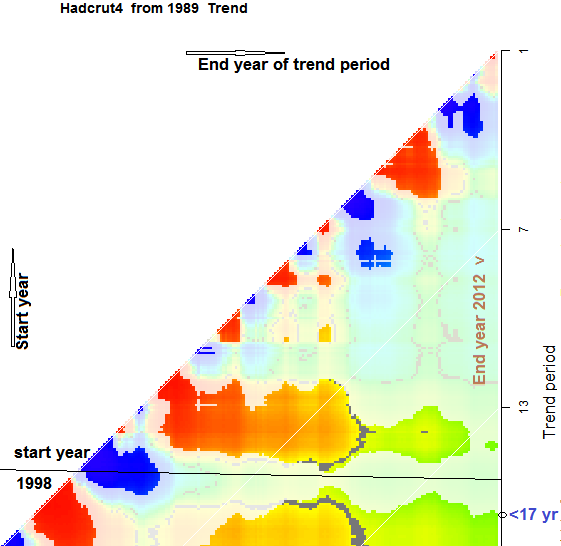
Here is a plot of Hadcrut 4 over the last 20 years. A snapshot of the relevant part is here:



The x axis is the recent end of the trend period, the y-axis is the past end (years). The right edge is Dec 2012. Fading represents trend that is not significantly different from zero using a AR(1) noise model at 95% (two-tail).

On the original plot, you can click anywhere to get information, and this helps in understanding the plot. Each color point represents a trend from year y to year x, and when you click, the red and blue dots on the time series plot at right show the interval, and the relevant statistical information is also shown. You can also move hte red and blue to change the interval and see the new trend and statistics.

The "17 years and four months" is the point on the right y axis where the color fades (near the bottom in the snapshot). The color of course, in the future, will respond to how warm it becomes. So I'm discussing what might happen to that color pattern as more data emerges on the right.

The first thing to note is the horizontal banding. This reflects the hot/cold pattern of years on the y-axis - ie in the '90s. The band near 14 on the axis is the cool years of 1999-2001. Trends that start there are likely to be positive and significant. The faded horizontal below is the warm year 1998. Trends that include that are smaller, and likely to not be significant. So a year or so ago, there was a jump from "13 years ago" to "17 years ago".

Except, of course, it was 16 years ago then. What has happened since is a result of the horizontal banding. The start year stays at about 1996 - it's in a sort of well. It can't go back much because trhe previous years are relatively cold, and including them will boost the significance strongly. And coming forward loses the warmup of 1997, which also boosts significance.

So unless it escapes from the well, we can expect "18 years and four months" next year. Will that happen?

Well, the gradual increase in time period improves significance even if the trend doesn't increase. So that helps get out of the well. What is likely, even without much warmong, is a reversal of the jump of a year ago. A switch to the 1999-2001 well, even though there would remain a band including 1998 which would be insignificant.

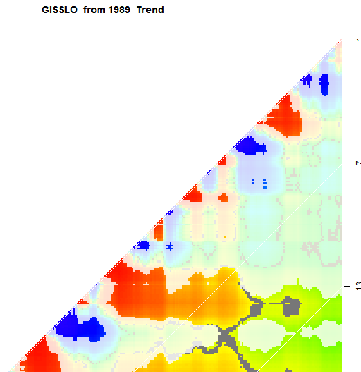
You can see this by looking instead at GISS. Here is the snapshot:



GISS did not make that transition, and so the significance period remains at a bit over 13 years. You can check other datasets on the trend gadget linked. You'll see the same horizontal banding.

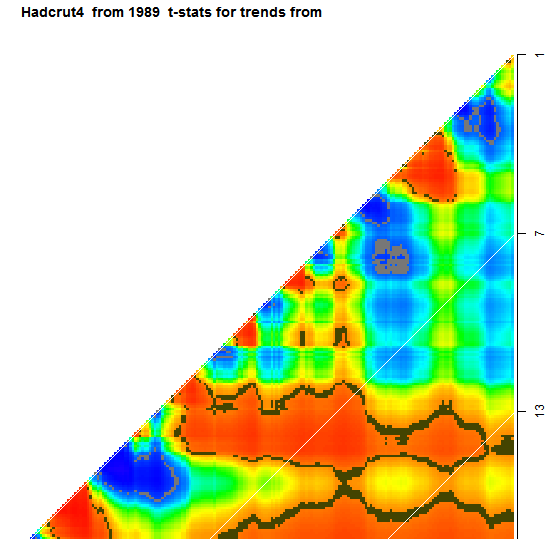
To get another view of what may be in store, you can look at the t-statistic. The critical 95% level is shown in brown. Here is a Had 4 snapshot:



Again you can see how constrained it is. It is close to significance near 14 years, and quite likely to go back there. There is a strong gradient at 17 years, so it can't start much before 1996. And earlier than 13 years, there are no new bands likely to emerge.

TempLS global temp up 0.06°C in May

The TempLS monthly anomaly for May 2013 was 0.480°C, compared with 0.418° in April.

Here is the spherical harmonics plot of the temperature distribution:



Warm in most of Asia and E Europe, with a cold spot in the middle..
And here is the map of stations reporting:

A climate blog reader

Google Reader is kaput at the end of June. I had been lazily eyeing alternatives, but I had also been looking into RSS systems, and it seemed that I could fairly easily write my own. It's a bit like re-inventing, but there are advantages. I used Google Reader a lot, though its limitations were painful. Improved searching is one aspiration. But if you read the feeds yourself, you can accumulate as much back data as you like.

Anyway, I found along the way that I could fairly easily compile an updated searchable list of comments on the main blogs that I was reading. My first attempt is below the jump. So far, I just have a few days data on the main Wordpress blogs. There are a lot of idiosyncracies, so I'll gradually extend it. When it has stabilized, I'll promote it to a page.




Update - I see the time ordering does not work in Chrome, though it does in Firefox. It's late here, so that will have to wait until morning. Although the time order is wrong, the rest seems OK. Fixed

Currently it shows all the comments that it is aware of. Updating is hourly. All times are GMT. You can click the buttons at the top to reorder. Main posts are indicated by a background color.

You can select subsets. You'll see four selection boxes top right. If they are empty, everything passes. Otherwise, for three of them, you can enter names, and only those will show. You can select commenters, blogs and threads. Time is different. You can select one or two times. If one, it will show only posts more recent. If two, it will show posts between those dates.

On the right you'll see a selection panel. The steps are:

1. Click on one of the selection boxes on left. It will turn pink to show it is active.
   
Make a name appear in the Result section on right (see below for how)
2. Click Enter. Your selection will be at the bottom of the list.
3. You can click delete to remove the top item in the active list.

There are two ways to enter a result. The simplest is to find a line displayed that has the aspect you want. Then click at that level on the red bar that is to the right of the table. You may have to click twice. Your selection should appear. If it is what you want, press enter.

The second way is to enter the first few letters in the text box, top right, and then click. If it gets something else, add more letters. Again, when it is right, press enter.

To make your selection show, just click one of the four column buttons, depending on the ordering you want.

If you want to select by blog, the posts and comments count separately (separate RSS files). Posts are indicated thus (WUWT_).

Issues

There has been more fuss than I expected. I managed to get my IP banned at Lucia's (promptly restored). The RSS files aren't all that standard. My outstanding problem is with SkS comments, which don't have dates. RSS files have a mix of old and new, and I use dates to distinguish. Even the SKS link numbering is non-unique. So I'll have to do a sort of dendrochronology. You'll see that There are chunks of SkS comments, with duplicates.

I'm only passing metadata (links etc) but even so, it's going to get big. After a couple of days the data file is 180Kb. I'm not sure yet how to handle that. At worst, it will be restricted to the last fortnight or so. The limitation is download time. This is all done in Javascript. I may end up downloading in chunks on request, as Reader did.

The main improvement planned is to allow (local) storage of the choices, which I've called environments. You could have several and switch between them.

And of course, to extend the range to blogs covered. Blogger is messier, but I'll tackle it next.

Of course, it all depends on my computer running every hour to catch and process the RSS files. On busier sites, the info is only there for a couple of hours. If my computer fails for any reason, there will be a gap. And it may all just get too hard and come to an end. No guarantees or promises. It's an experiment.