Friday, September 29, 2017

Nested gridding, Hadcrut, and Cowtan/Way .

Update I had made an error in coding for the HADCRUT/C&W example - see below. The agreement with C&W is now much improved.

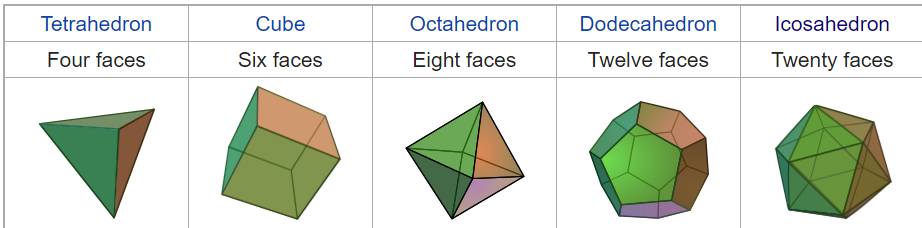
In my previous post, I introduced the idea of hierarchical, or nested gridding. In earlier posts, eg here and here, I had described using platonic solids as a basis for grids on the sphere that were reasonably uniform, and free of the pole singularities of latitude/longitude. I gave data files for icosahedral hexagon meshes of various degrees of resolution, usually proceeding by a factor of two in cell number or length scale. And in that previous post, I emphasised the simplicity of a scheme for working out which cell a point belonged by finding the nearest centre point. I foreshadowed the idea of embedding each such grid in a coarser parent, with grid averaging proceeding downward, and using the progressive information to supply estimates for empty cells.

The following graph from HADCRUT illustrates the problem. It shows July 2017 temperature anomalies on a 5°x5° grid, with colors for cells that have data, and white otherwise. They average the area colored, and omit the rest from the average. As I often argue, as a global estimate, this effectively replaces the rest by the average value. HADCRUT is aware of this, because they actually average by hemispheres, which means the infilling is done with the hemisphere average rather than global. As they point out, this has an important benefit in earlier years when the majority of missing cells were in the SH, which was also behaving differently, so the hemisphere average is more eappropriate than global. On the right, I show the same figure, but this time with my crude coloring in (with Paint) of that hemisphere average. You can assess how appropriate the infill is:


A much-discussed paper by Cowtan and Way 2013 noted that this process led to bias in that the areas thus infilled tended not to have the behaviour of the average, but were warming faster, and this was underestimated particularly since 2000 because of the Arctic. They described a number of remedies, and I'll concentrate on the use of kriging. This is a fairly elaborate geostatistical interpolation method. When applied, HADCRUT data-based trends increased to be more in line with other indices which did some degree of interpolation.

I think the right way to look at this is getting infilling right. HADCRUT was on the right track in using hemisphere averages, but it should be much more local. Every missing cell should be assigned the best estimate based on local data. This is in the spirit of spatial averaging. The cells are chosen as regions of proximity to a finite number of measurement points, and are assigned an average from those points because of the proximity. Proximity does not end at an artificial cell boundary.

In the previous post, I set up a grid averaging based on an inventory of about 11000 stations (including GHCN and ERSST) but integrated not temperature but a simple function sin(latitude)^2, which should give 1/3. I used averaging omitting empty cells, and showed that at coarse resolution the correct value was closely approximated, but this degraded with refinement, because of the accession of empty cells. I'll now complete that table using nested integration with hexagonal grid. At each successive level, if a cell is empty, it is assigned the average value of the smallest cell from a previous integration that includes it. (I have fixed the which.min error here too; it made little difference).

levelNumcellsSimple averageNested average
11320.32920.3292
221220.33110.3311
332720.32750.3317
444820.32560.3314
5510820.32060.3317
6619220.31670.332
7736320.3110.3313
8876820.30960.3315


The simple average shows that there is an optimum; a grid fine enough to resolve the (small) variation, but coarse enough to have data in most cells. The function is smooth, so there is little penalty for too coarse, but a larger one for too fine, since the areas of empty cells coincides with the function peak at the poles. The merit of the nested average is that it removes this downside. Further refinement may not help very much, but it does no harm, because a near local value is always used.

The actual coding for nested averaging is quite simple, and I'll give a more complete example below.

HADCRUT and Cowtan/Way

Cowtan and Way thankfully released a very complete data set with their paper, so I'll redo their calculation (with kriging) with nested gridding and compare results. They used HADCRUT 4.1.1.0, data ending at end 2012. Here is a plot of results from 1980, with nested integration of the HADCRUT gridded data at centres (but on a hex grid). I'm showing every even step as hier1-4, with hier4 being the highest resolution at 7682 cells. All anomalies relative to 1961-90..


UpdateI had made an error in coding for the HADCRUT/C&W example - see code. I had used which.min instead of which.max. This almost worked, because it placed locations in the cells on the opposite side of the globe, consistently. However, the result is now much more consistent with C&W. With refining, the integrals now approach from below, and also converge much more tightly.

The HADCRUT 4 published monthly average (V4.1.1.0) is given in red, and the Cowtan and Way Version 1 kriging in black. The nested integration makes even more difference than C&W, mainly in the time from 1995 to early 2000's. Otherwise, a As with C&W, it adheres closely to HADCRUT in earlier years, when presumably there isn't much bias associated with the missing data. C&W focussed on the effect on OLS trends, particularly since 1/1997. Here is a table, in °C/Century:

Trend 1997-2012Trend 1980-2012
HAD 40.4621.57
Hier10.9021.615
Hier20.9291.635
Hier30.9671.625
Hier40.9561.624
C&W krig0.971.689


Convergence is very good to the C&W trend I calculate. In their paper, for 1997-2012 C&W give a trend of 1.08 °C/Cen (table III) which would agree very well with the nested results. C&W used ARMA(1,1) rather than OLS, but the discrepancy seems too large for that.Update: Kevin Cowtan has explained the difference in a comment below.

Method and Code

This is the code for the integration of the monthly sequence. I'll omit the reading of the initial files and the graphics, and assume that we start with the HADCRUT 4.1.1.0 gridded 1980-2012 data reorganised into an array had[72,36,12,33] (lon,lat,month,year). The hexmin[[]] lists are as described and posted previously. The 4 columns of $cells are the cell centres and areas (on sphere). The first section is just making pointer lists from the anomaly data into the grids, and from each grid into its parent. If you were doing this regularly, you would store the pointers and just re-use as needed, since it only has location data. The result is the gridpointer and datapointer lists. The code takes a few seconds.
monthave=array(NA,c(12,33,8)) #array for monthly averages 
datapointer=gridpointer=cellarea=list(); g=0;
for(i in 1:8){ # making pointer lists for each grid level
 g0=g;  # previous g
 g=as.matrix(hexmin[[i]]$cells); ng=nrow(g);
 cellarea[[i]]=g[,4]
 if(i>1){ # pointers to coarser grid i-1
  gp=rep(0,ng)
  for(j in 1:ng)gp[j]=which.max(g0[,1:3]%*%g[j,1:3])
  gridpointer[[i]]=gp
 }
 y=inv; ny=nrow(y); dp=rep(0,ny) #  y is list of HAD grid centres in 3D cartesian
 for(j in 1:ny) dp[j]=which.max(g[,1:3]%*%y[j,])
 datapointer[[i]]=dp  # datapointers into grid i
}
Update: Note the use of which.max here, which is the key instruction locating points in cells. I had originally used which.min, which actually almost worked, because it places ponts on the opposite side of the globe, and symmetry nearly makes that OK. But not quite. Although the idea is to minimise the distance, that is implemented as maximising the scalar product.

The main data loop just loops over months, counting and adding the data in each cell (using datapointer); forming a cell average. It then inherits from the parent grid values (for empty cells) from the parent average vector using gridpointer to find the match, so at each ave is complete. There is an assumption that the coarsest level has no empty cells. It is then combined with area weighting (cellarea, from hexmin) for the monthly average. Then on to the next month. The result is the array monthave[month, year, level] of global averages.
for(I in 1:33)for(J in 1:12){ # looping over months in data from 1980
 if(J==1)print(Sys.time())
 ave=rep(NA,8)  # initialising
 #tab=data.frame(level=ave,Numcells=ave,average=ave)
 g=0
 for(K in 1:8){ # over resolution levels
  ave0=ave
  integrand=c(had[,,J,I+130])  # Set integrand to HAD 4 for the month 
  area=cellarea[[K]]; 
  cellsum=cellnum=rep(0,length(area))  # initialising
  dp=datapointer[[K]]
  for(i in 1:n){  # loop over "stations"
   ii=integrand[i]
   if(is.na(ii))next  # no data in cell
   j=dp[i]
   cellsum[j]=cellsum[j]+ii
   cellnum[j]=cellnum[j]+1
  }
  j=which(cellnum==0) # cells without data
  gp=gridpointer[[K]]
  if(K>1)for(i in j){cellnum[i]=1;cellsum[i]=ave0[gp[i]]}
  ave=cellsum/cellnum # cell averages
  Ave=sum(ave*area)/sum(area) # global average (area-weighted)
  if(is.na(Ave))stop("A cell inherits no data")
  monthave[J,I,K] = round(Ave,4) # weighted average
 }
}# end I,J

Data

Moyhuhexmin has the hex cell data and was given in the earlier post. I have put a new zipped ascii version here


Thursday, September 28, 2017

Simple use of a complex grid - Earth temperature.

This is a follow-up to my last post, which refined ideas from an earlier post on using platonic solids as a basis for grids on the sphere that were reasonably uniform, and free of the pole singularities of latitude/longitude. I gave data files for use, as I did with an earlier post on a special case, the cubed sphere.

The geometry involved can be complicated, but a point I made in that last post was that users need never deal with the complexity. I gave a minimal set of data for grids of varying resolution, which basically recorded the mid-points of the cells, and their area. That is all you need to make use of them.

I should add that I don't think the hexagon method I recommend is a critical improvement over, say, the cubed sphere method. Both work well. But since this method of application is the same for any variant, just using cell centres and areas in the same way, there is no cost in using the optimal.

In this post, I'd like to demonstrate that with an example, with R code for definiteness. I'd also like to expand on the basic idea, which is that near-regular grids of any complexity have he Voronoi property, which is that cells are the domain of points closest to the mid-points. That is why mid-point location is sufficient information. I can extend that to embedding grids in grids of lower resolution; I will recommend a method of hierarchical integration in which empty cells inherit estimates from the most refined grid that has information for their area. I think this is the most logical answer to the empty cell problem.

In the demonstration, I will take the inventory of stations that I use for TempLS. It has all GHCN V3 stations together with a selection of ERSST cells, treated as stations located at grid centres. It has 10997 locations. I will show how to bin these, and use the result to do a single integration of data on those points.

I start with calling the data for the inventory ("invo.sav") (posted in the dataset for cubed sphere above). Then I call the Moyhuhexmin data that I posted in the last post. I am going to do the integration over all 8 resolution levels, so I loop over variable K, collecting results in ave[]:
load("invo.sav")
load("Moyhuhexmin.sav")
ave=rep(NA,8) # initialising
for(K in 1:8){
 h=hexmin[[K]]  # dataframe for level K
 g=as.matrix(h$cells) # 3D coords of centres, and areas
 y=invo$z; n=nrow(y);  # invo$z are stations; 
 pointer=rep(0,n)
This is just gathering the information. g and y are the two sets of 3D cartesian coordinates on the sphere to work with. Next I locate y in the cells which have centre g:
 pointer=rep(0,n)
 for(i in 1:n) pointer[i]=which.min(g[,1:3]%*%y[i,]) # finding closest g to y 
If this were a standalone calculation, I wouldn't have done this as a separate loop. But the idea is that, once I have found the pointers, I would  store them as a property of the stations, and never have to do this again. Not that it is such a pain; although I discussed last time a multi-stage process, first identifying the face and then searching that subset, in fact with near 11000 nodes and 7682 cells (highest resolution), the time taken is still negligible - maybe 2 seconds on my PC.

Now to do an actual integration. I'll use a simple known function, where one would normally use temperature anomalies assigned to a subset of stations y. I'll use the y-coord in my 3D, which is sin(latitude),, and sunce that has zero integral, I'll integrate the square. The answer should be 1/3.
integrand=y[,2]^2
area=g[,4]; 
cellsum=cellnum=rep(0,nrow(g))  # initialising
for(i in 1:n){
 j=pointer[i]
 cellsum[j]=cellsum[j]+integrand[i]
 cellnum[j]=cellnum[j]+1
}
area[] is just the fourth column of data from hexmin; it is the area of each cell on the sphere. cellsum[] with be the sum of integrand values in the cell, and cellnum[] the count (for averaging). This is where the pointers are used. The final stage is the weighted summation:
o=cellnum>0 # cells with data
ave[K] = sum(cellsum[o]*area[o]/cellnum[o])/sum(area[o]) # weighted average
} # end of K loop
This is, I hope, fairly obvious R stuff. o[] marks cells with data which are the only ones included in the sum. area[o] are the weights, and to get the averages I divide by the sum of weights. This is just conventional grid averaging.

Integration results

Here are the results of grid integration of sin^2(lat) at various resolution levels:

levelNumber of cellsaverage
1320.3292
21220.3311
32720.3275
44820.3256
510820.3206
619220.3167
736320.3108
876820.3096
The exact answer is 1/3. This was reached at fairly coarse resolution, which is adequate for this very smooth function. At finer resolution, empty cells are an increasing problem. Simple averaging ignoring empty cells effectively assigns to those eells the average of the rest. Because the integrand has peak value 1 at the poles, where many cells are empty, those cells are assigned a value of about 1/3, when they really should be 1. That is why the integral diminishes with increasing resolution. It is also why the shrinkage tapers off, because once most cells in the region are empty, further refinement can't make much difference.

Empty cells and HADCRUT

This is the problem that Cowtan and Way 2013 studied with HADCRUT. HADCRUT averages hemispheres separately, so they effectively infill empty cells with hemisphere averages. But Arctic areas especially are warming faster than average, and HADCRUT tends to miss this. C&W tried various methods of interplating, particularly polar values, and got what many thought was an improvement, more in line with other indices. I showed at the time that just averaging by latitude bands went a fair way in the same direction.

With the new grid methods here, that can be done more systematically. The Voronoi based matching can be used to embed grids in grids of lower resolution, but fewer empty cells. Integrtaion can be done starting with a coarse grid, and then going to higher resolution. Infilling of an empty cell can be done with the best value from the heirarchy.

I use an alternative diffusion based interpolation as one of the four methods for TempLS. It works very well, and gives results similar to the other two of the three best (node-nased triangular mesh and spherical harmonics). I have tried variants of the heirarchical method, with similar effect.

Next

In the next post, I will check out the hierarchical method applied to this simple example, and also to HADCRUT4 gridded version. I'm hoping from a better match with Cowtan and Way.


Tuesday, September 26, 2017

The best grid for Earth temperature calculation.

Earlier this month, I wrote about the general ideas of gridding, and how the conventional latitude/longitude grids were much inferior to grids that could be derived from various platonic solids. The uses of gridding in calculating temperature (or other field variables) on a sphere are
  1. To gather like information into cells of known area
  2. To form an area weighted sum or average, representative of the whole sphere
  3. a necessary requirement is that it is feasible to work out in which cell an arbitrary location belongs
So a good grid must have cells small enough that variation within them has little effect on the result ("like"), but large enough that they do significant gathering. It is not much use having a grid where most cells are empty of data. This leads to two criteria for cells that balance these needs:
  • The cells should be of approximately equal area.
  • The cells should be compact, so that cells of a given area can maximise "likeness".
Lat/lon fails because:
  • cells near poles are much smaller
  • the cells become long and thin, with poor compactness
I showed platonic solid meshes with triangles and squares that are much less distorted, and with more even area distribution, Clive Best, too, has been looking at icosahedra. I have also been looking at ways of improving area uniformity. But I haven't been thinking much about compactness. The ideal there is a circle. Triangles deviate most; rectangles are better, if nearly square. But better still are regular hexagons, and that is my topic here.

With possibly complex grids, practical usability is important. You don't want to keep having to deal with complicated geometry. With the cubed sphere, I posted  here a set of data which enables routine use with just lookup. It includes a set of meshes with resolution increasing by factors of 2. The nodes have been remapped to optimise area uniformity. There is a lookup process so that arbitrary points can be celled. But there is also a list showing in which cell the stations of the inventory that I use are found. So although the stations that report vary each month, there is a simple geometry-free grid average process
  • For each month, sort the stations by cell label
  • Work out cell averages, then look up cell areas for weighted sum.
I want to do that here for what I think is an optimal grid.

The optimal grid is derived from the triangle grid for icosahedra, although it can also be derived from the dual dodecahedron. If the division allows, the triangles can be gathered into hexagons, except near vertices of the icosahedron, where pentagons will emerge. This works provided the triangles faces are initially trisected, and then further divided. There will be 12 pentagons, and the rest hexagons. I'll describe the mapping for uniform sphere surface area in an appendix.

Lookup

I have realised that the cell finding process can be done simply and generally. Most regular or near-regular meshes are also Voronoi nets relative to their centres. Thatis, a cell includes the points closest to its centre, and not those closer to any other centre. So you can find the cell for a point by simply looking for the closest cell center. For a sphere that is even easier; it is the centre for which the scalar product (cos angle) of 3D coordinates is greatest.

If you have a lot of points to locate, this can still be time-consuming, if mechanical. But it can be sped up. You can look first for the closest face centre (of the icosahedron). Then you can just check the cells within that face. That reduces the time by a factor of about 20.

The grids

Here is a WebGL depiction of the results. I'm using the WebGL facility, V2.1. The sphere is a trackball. You can choose the degree of resolution with the radio buttons on the right; hex122, for example, means a total of 122 cells. They progress with factors of approx 2. The checkboxes at the top let you hide various objects. There are separate objects for red, yellow and green, but if you hide them all, you see just the mesh. The colors are designed to help see the icosahedral pattern. Pentagons are red, surrounded by a ring of yellow.


The grid imperfections now are just a bit of distortion near the pentagons. This is partly because I have forced them to expand to have simiar area to the hexagons. For grid use, the penalty is just a small loss of compactness.

Data

The data is in the form of a R save file, for which I use the suffix .sav. There are two. One here is a minimal set for use. It includes the cell centre locations, areas, and a listing of the cells within each face, for faster search. That is all you need for routine use. There is a data-frame with this information for each of about 8 levels of resolution, with maximum 7682 cells (hex7682). There is a doc string.

The longer data set is here. This has the same levels, but for each there are dataframes for cells, nodes, and the underlying triangular mesh. A dataframe is just R for a matrix that can have columns of various types, suitably labelled. It gives all the nodes of the triangular mesh, with various details. There are pointers from one set to another. there is also a doc string with details.

Appendix - equalising area

As I've occasionally mentioned, I've spent a lot of time on this interesting math problem. The basic mapping from platonic solid to sphere is radial projection. But that distorts areas that were uniform on the solid. Areas near the face centres are projected further (thinking of the solid as within the sphere) and grow. There is also, near the edges, an effect due to the face plane slanting differently to the sphere (like your shadow gets smaller when the sun is high). These distortions get worse when the solid is further from spherical.

I counter this with a mapping which moves the mesh on the face towards the face centre. I initially used various polynomials. But now I find it best to group the nodes by symmetry - subsets that have to move in step. Each has one (if on edge) or two degrees of freedom. Then the areas are also constrained by symmetry, and can be grouped. I use a Newton-Raphson method (actually secant) to move the nodes so that the triangles have area closest to the ideal, which is the appropriate fraction of the sphere. There are fewer degrees of freedom than areas, so it is a kind of regression calculation. It is best least squares, not exact. You can check the variation in areas; it gets down to a few percent.


Tuesday, September 19, 2017

GISS August up 0.01°C from July.

GISS showed a very small rise, going from 0.84°C in July to 0.85°C in August (GISS report here). TempLS mesh showed a very slight fall, which I posted at 0.013°C, although with further data is is now almost no change at all. I see that GISS is now using ERSST V5, as TempLS does.

The overall pattern was similar to that in TempLS. Warm almost everywhere, with a big band across mid-latitude Eurasia and N Africa. Cool in Eastern US and high Arctic, which may be responsible for the slowdown in ice melting..

As usual here, I will compare the GISS and previous TempLS plots below the jump.

Monday, September 18, 2017

Grids, Platonic solids, and surface temperature (and GCMs)

This follows a series, predecessor here, in which I am looking at ways of dealing with surface variation of Earth's temperature, particularly global averaging. I have written a few posts on the cubed sphere, eg here. I have also shown some examples of using an icosahedron, as here. Clive Best has been looking at similar matters, including use of icosahedron. For the moment, I'd like to write rather generally about grids and ways of mapping the sphere.

Why grids?

For surface temperature, grids are commonly used to form local averages from data, which can then be combined with area weighting to average globally. I have described the general considerations here. All that is really required is any subdivision of reasonable (compact) shapes. They should be small enough that the effect of variation within is minimal, but large enough that there is enough data for a reasonable estimate. So they should be of reasonably equal area.

The other requirement, important later for some, is that any point on the sphere can be associated with the cell that contains it. For a regular grid like lat/lon, this is easy, and just involves conversion to integers. So if each data point is located, and each cell area is known, that is all that is needed. As a practical matter, once the cell locations are known for an inventory of stations, the task of integrating the subset for a given month is just a look-up, whatever the geometry.

I described way back a fairly simple subdivision scheme that works for this. Equal latitude bands are selected. Then each band is divided as nearly as possible into square elements (on the sphere). The formula for this division can then be used to locate arbitrary points within the cells. I think this is all that is required for surface averaging.

However, for anything involving partial differentiation, such as finite element or GCM modelling, more is required. Fluxes between cells need to be measured, so hey have to line up. Nodes have to be related to each cell they abut. This suggests regular grids. In my case, I sometimes want to use a kind of diffusive process to estimate what is happening in empty cells. Again, regular is better.

Platonic solids

Something that looks a bit like a sphere and is easy to fit with a regular grid is a Platonic solid. There are five of them - I'll show the Wiki diagram:


Regular means that each side has the same length, and each face is a congruent regular polygon. The reason why there are only five is seen if you analyse what has to happen at vertices (Wiki):

Friday, September 8, 2017

August global surface temperature down 0.013°C

TempLS mesh anomaly (1961-90 base) was down from 0.69°C in July to 0.677°C in August. This very small drop compares with the small rise of 0.038°C in the NCEP/NCAR index, and a bigger rise (0.12) in the UAH LT satellite index. The August value is less than August 2015 or 2016, but higher than 2014.

There was a moderate fall in Antarctica, which as usual affects TempLS mesh and GISS more than others. I'd expect NOAA and HADCRUT to show increases for August. Regionally, the Old World was mostly warm; US was cold cental and East, but N Canada was warm. S America mostly warm (still awaiting a few countries). :


Thursday, September 7, 2017

August NCEP/NCAR global anomaly up 0.038°C

In the Moyhu NCEP/NCAR index, the monthly reanalysis average rose from 0.299°C in July to 0.337°C in August, 2017. The results were late this month; for a few days NCEP/NCAR was not posting new results. It was a very up and down month; a dip at at the start, then quite a long warm period, and then a steep dip at the end. Now that a few days in September are also available, there is some recovery from that late dip. August 2017 was a bit cooler than Aug 2016, but warmer than 2015.

It was cool in Eastern US, but warm in the west and further north. Cool in Atlantic Europe, but warm further east. Mostly cool in Antarctica.