Methods of integrating temperature anomalies on the sphere

A few days ago, I described a new method for integrating temperature anomalies on the globe, which I called FEM/LOESS. I think it may be the best general purpose method so far. In this post I would like to show how well it works within TempLS, with comparisons with other advanced methods. But first I would like to say a bit more about the mathematics of the method. I'll color it blue for those who would like to skip.

Mathematics of FEM/LOESS

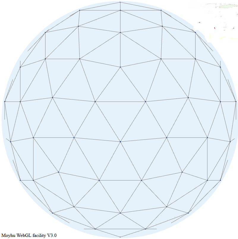
It's actually a true hybrid of the finite element method (FEM) and LOESS (locally estimated scatterplot smoothing). In LOESS a model is fitted locally by regression, usually to get a central value. In FEM/LOESS, the following least squares parameter fit is made:

The standard FEM approximate function is f(z)=ΣaᵢBᵢ(z) where z is location on the sphere, B are the basis functions described in the previous post, and aᵢ are the set of coefficients to be found by fitting to a set of observations that I will call y(z). The LS target is

SS=∫(f(z)-y(z))^2 dz

This has to be estimated knowing y at a discrete points (stations). In FEM style, the integral is split into integrals over elements, and then within elements the integrand is estimated as mean (f(zₖ)-y(zₖ))^2 over points k. One might question whether the sum within elements should be weighted, but the idea is that the fitted f() takes out the systematic variation, so the residuals should be homogeneous, and a uniform mean is correct.

So differentiating wrt a to minimise:
∫(f(z)-y(z))Bᵢ(z) dz = 0
Discretising:

Σₘ Eₘ (ΣₖBᵢ(zₖ)Bₙ(zₖ)aₙ)/(Σₖ1) = Σₘ Eₘ (ΣₖBᵢ(zₖ)yₖ)/(Σₖ1)

The first summation is over elements, and E are their areas. In FEM style, the summations that follow are specific to each element, and for each E include just the points zₖ within that element, and so the basis functions in the sum are those that have a node within or on the boundary if that element. The denominators Σₖ1 are just the count of points within each element. It looks complicated but putting it together is just the standard FEM step of assembling a mass matrix.

In symbols,this is the regression equation
H a = B^* w B a = B^* w y
where B is the matrix of basis functions evaluated at zₖ, B^* transpose, diagonal matrix w the weights Σₘ/(Σₖ1) (area/count), y the vector of readings, and a the vector of unknown coefficients.

To integrate a specific y, this has to be solved for a:
a=H^-1B^* w y
and then ΣaᵢBᵢ(z) integrated on the globe
Int = ΣaᵢIᵢ where Iᵢ is the integral of function Bᵢ,

H is generally positive definite and sparse, so the inversion is done with conjugate gradients, using the diagonal as preconditioner.

For TempLS I need not an integral but weights. So I have to calculate

wt = I H^-1B^* w

It sounds hard, but it is a well trodden FEM task, and is computationally quite fast. In all this a small multiple of a Laplacian matrix is added to H to ensure corresponding infilling of empty or inadequately constrained cells.

Comparisons

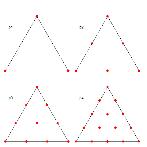
I ran TempLS using the FEM/LOESS weighting with 9 modes, h2p2, h2p3, h2p4,...h43,h4p4. I calculated the RMS of differences between monthly averages, pairwise, for the years 1900-2019, and similar differences between and within the advanced methods MESH, LOESS and INFILL (see here for discussion, and explanation of the h..p.. notation). Here is a table of results, of RMS difference in °C, multiplied by 1000:

	MESH	LOESS	INFILL	h2p2	h3p2	h4p2	h5p2	h2p3	h3p3	h4p3	h5p3	h2p4	h3p4	h4p4	h5p4	h2p5	h3p5	h4p5	h5p5
MESH	0	18	19	26	20	19	19	21	18	17	19	18	17	17	19	19	19	19	22
LOESS	18	0	25	24	22	19	22	20	22	20	23	19	22	21	24	22	23	24	27
INFILL	19	25	0	27	19	17	14	21	14	13	11	17	11	11	10	14	11	10	12
h2p2	26	24	27	0	24	25	26	21	24	24	26	22	25	25	26	26	26	27	28
h3p2	20	22	19	24	0	17	16	16	11	16	17	16	12	17	18	16	17	17	21
h4p2	19	19	17	25	17	0	14	15	12	8	16	12	13	10	14	14	16	17	20
h5p2	19	22	14	26	16	14	0	17	11	11	6	13	10	10	12	0	6	8	12
h2p3	21	20	21	21	16	15	17	0	16	16	19	10	17	17	19	17	19	20	23
h3p3	18	22	14	24	11	12	11	16	0	10	11	12	6	10	12	11	11	13	16
h4p3	17	20	13	24	16	8	11	16	10	0	11	11	9	4	9	11	11	12	16
h5p3	19	23	11	26	17	16	6	19	11	11	0	15	9	9	10	6	0	4	8
h2p4	18	19	17	22	16	12	13	10	12	11	15	0	13	12	15	13	15	16	20
h3p4	17	22	11	25	12	13	10	17	6	9	9	13	0	8	10	10	9	10	14
h4p4	17	21	11	25	17	10	10	17	10	4	9	12	8	0	6	10	9	10	14
h5p4	19	24	10	26	18	14	12	19	12	9	10	15	10	6	0	12	10	9	12
h2p5	19	22	14	26	16	14	0	17	11	11	6	13	10	10	12	0	6	8	12
h3p5	19	23	11	26	17	16	6	19	11	11	0	15	9	9	10	6	0	4	8
h4p5	19	24	10	27	17	17	8	20	13	12	4	16	10	10	9	8	4	0	6
h5p5	22	27	12	28	21	20	12	23	16	16	8	20	14	14	12	12	8	6	0

The best agreement between the older methods is between MESH and LOESS at 18. Agreement between the higher order FEM results is much better. Agreement of FEM with MESH is a little better, with LOESS a little worse. The agreement with INFILL is better again, but needs to be discounted somewhat. The reason is that in earlier years there is a large S Pole region without data. Both INFILL and FEM deal with this with Laplace interpolation, so I think that spuriously enhances the agreement.
As will be seen later, there is a change in the matchings at about 1960, when Antarctic data becomes available. So I did a similar table just for the years since 1960:

	MESH	LOESS	INFILL	h2p2	h3p2	h4p2	h5p2	h2p3	h3p3	h4p3	h5p3	h2p4	h3p4	h4p4	h5p4	h2p5	h3p5	h4p5	h5p5
MESH	0	11	11	23	17	16	14	18	13	12	12	15	12	11	10	14	12	12	16
LOESS	11	0	10	19	14	12	10	14	10	9	9	10	9	8	9	10	9	10	14
INFILL	11	10	0	21	16	16	13	17	13	12	11	15	11	10	9	13	11	10	13
h2p2	23	19	21	0	20	20	20	18	20	20	20	18	20	20	21	20	20	20	22
h3p2	17	14	16	20	0	15	15	13	10	14	15	13	11	14	16	15	15	15	19
h4p2	16	12	16	20	15	0	12	12	10	7	14	9	10	9	13	12	14	16	20
h5p2	14	10	13	20	15	12	0	15	11	9	6	11	10	10	11	0	6	8	13
h2p3	18	14	17	18	13	12	15	0	12	13	16	10	13	14	16	15	16	17	20
h3p3	13	10	13	20	10	10	11	12	0	9	12	8	6	9	11	11	12	13	17
h4p3	12	9	12	20	14	7	9	13	9	0	10	9	7	4	8	9	10	11	16
h5p3	12	9	11	20	15	14	6	16	12	10	0	13	9	9	9	6	0	4	9
h2p4	15	10	15	18	13	9	11	10	8	9	13	0	9	9	12	11	13	14	18
h3p4	12	9	11	20	11	10	10	13	6	7	9	9	0	7	9	10	9	11	15
h4p4	11	8	10	20	14	9	10	14	9	4	9	9	7	0	6	10	9	10	15
h5p4	10	9	9	21	16	13	11	16	11	8	9	12	9	6	0	11	9	9	13
h2p5	14	10	13	20	15	12	0	15	11	9	6	11	10	10	11	0	6	8	13
h3p5	12	9	11	20	15	14	6	16	12	10	0	13	9	9	9	6	0	4	9
h4p5	12	10	10	20	15	16	8	17	13	11	4	14	11	10	9	8	4	0	7
h5p5	16	14	13	22	19	20	13	20	17	16	9	18	15	15	13	13	9	7	0

Clearly the agreement is much better. The best of the older methods is between LOESS and INFILL at 10. But agreement between high order FEM methods is better. Now it is LOESS that agrees well with FEM - better than the others. Of course in assessing agreement, we don't know which is right. It is possible that FEM is the best, but not sure.

Here are some time series graphs. I'll show a time series graph first, but the solutions are too close to distinguish much.





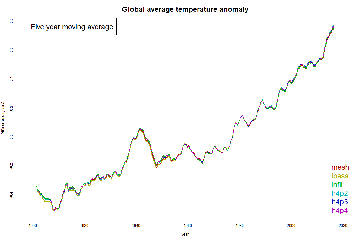
Difference plots are more informative. These are made by subtracting one of the solutions from the others. I have made plots using each of MESH, LOESS and INFILL as reference. You can click the buttons below the plot to cycle through.



There is a region of notably good agreement between 1960 and 1990. This is artificial, because that is the anomaly base period, so all plots have mean zero there. Still, they are unusually aligned in slope.

Before 1960, LOESS deviates from the FEM curves, MESH less, and INFILL least. The agreement of INFILL probably comes from the common use of Laplace interpolation for the empty Antarctic region. In the post 1990 period, it is LOESS which best tracks with FEM.

However, I should note that no discrepancies exceed about 0.02°C.

Next steps

After further experience, I will probably make FEM/LOESS my frontline method.

GISS September global unchanged from August.

The GISS V4 land/ocean temperature anomaly stayed at 0.90°C in September, same as August. It compared with a 0.043deg;C fall in TempLS V4 mesh

The overall pattern was similar to that in TempLS. Warm in Africa, N of China, Eastern US, NE Pacific, Alaska/Arctic. Cool over Urals, in West Coast USA and Atlantic Canada. Mostly cool in Antarctica.

As usual here, I will compare the GISS and earlier TempLS plots below the jump.

New FEM/LOESS method of integrating temperature anomalies on the globe

Update Correction to sensitivity to rotation below

Yet another post on this topic, which I have written a lot about. It is the the basis of calculation of global temperature anomaly, which I do every month with TempLS. I have developed three methods that I consider advanced, and I post averages using each here (click TempLS tab). They agree fairly well, and I think they are all satisfactory (and better than the alternatives in common use). The point of developing three was partly that they are based on different principles, and yet give concordant results. Since we don't have an exact solution to check against, that is the next best thing.

So why another one? Despite their good results, the methods have strong points and some imperfections. I would like a method that combines the virtues of the three, and sheds some faults. A bonus would be that it runs faster. I think I have that here. I'll call it the FEM method, since it makes more elaborate use of finite element ideas. I'll first briefly describe the existing methods and their pros and cons.

Mesh method

This has been my mainstay for about eight years. For each month an irregular triangular mesh (convex hull) is drawn connecting the stations that reported. The function formed by linear interpolation within each triangle is integrated. The good thing about the method is that it adapts well to varying coverage, giving the (near) best even where sparse. One bad thing is the different mesh for each month, which takes time to calculate (if needed) and is bulky to put online for graphics. The time isn't much; about an hour in full for GHCN V4, but I usually store geometry data for past months, which can reduce process time to a minute or so. But GHCN V4 is apt to introduce new stations, which messes up my storage.

A significant point is that the mesh method isn't stochastic, even though the data is best thought of as having a random component. By that I mean that it doesn't explicitly try to integrate an estimated average, but relies o exact integration to average out. It does, generally, very well. But a stochastic method gives more control, and is alos more efficient.

Grid method with infill

Like most people, I started with a lat/lon grid, averaging station values within each cell, and then an area-weighted average of cells. This has a big problem with empty cells (no data) and so I developed infill schemes to estimate those from local dat. Here is an early description of a rather ad hoc method. Later I got more systematic about it, eventually solving a Laplace equation for empty cell regions, using data cells as boundary conditions.

The method is good for averaging, and reasonably fast. It is stochastic, in the cell averaging step. But I see it now in finite element terms, and it uses a zero order representation within the cell (constant), with discontinuity at the boundary. In FEM, such an element would be scorned. We can do better. It is also not good for graphics.,

LOESS method

My third, and most recent method, is described here. It starts with a regular icosahedral grid of near uniform density. LOESS (local weighted linear regression) is used to assign values to the nodes of that grid, and an interpolation function (linear mesh) is created on that grid which is either integrated or used for graphics. It is accurate and gives the best graphics.

Being LOESS, it is explicitly stochastic. I use an exponential weighting function derived from Hansen's spatial correlation decay, but a more relevant cut-off is that for each node I choose the nearest 20 points to average. There are some practical reasons for this. An odd side effect is that about a third of stations do not contribute; they are in dense regions where they don't make the nearest 20 of any node. This is in a situation of surfeit of information, but it seems a pity to not use their data in some way.

The new FEM method.

I take again a regular triangle grid based on subdividing the icosahedron (projected onto the sphere). Then I form polynomial basis functions of some order (called P1, P2 etc in the trade). These have generally a node for each function, of which there may be several per triangle element - the node arrangement within triangles are shown in a diagram below. The functions are "tent-like", and go to zero on the boundaries, unless the node is common to several elements, in which case it is zero on the boundary of that set of elements and beyond. They have the property of being one at the centre and zero at all other nodes, so if you have a function with values at the node, multiplying those by the basis functions and adding forms a polynomial interpolation of appropriate order, which can be integrated or graphed. Naturally, there is a WebGL visualisation of these shape functions; see at the end.

The next step is somewhat nonstandard FEM. I use the basis functions as in LOESS. That is, I require that the interpolating will be a best least squares fit to the data at its scattered stations. This is again local regression. But the advantage over the above LOESS is that the basis functions have compact support. That is, you only have to regress, for each node, data within the elements of which the node is part.

Once that is done, the regression expressions are aggregated as in finite element assembly, to produce the equivalent of a mass matrix which has to be inverted. The matrix can be large but it is sparse (most element zero). It is also positive definite and well conditioned, so I can use a preconditioned conjugate gradient method to solve. This converges quickly.

Advantages of the method

• Speed - binning of nodes is fast compared to finding pairwise distances as in LOESS, and furthermore it can be done just once for the whole inventory. Solution is very fast.
• Graphics - the method explicitly creates an interpolation method.
• Convergence - you can look at varying subdivision (h) and polynomial order of basis (p). There is a powerful method in FEM of hp convergence, which says that if you improve h and p jointly on some way, you get much faster convergence than improving one with the other fixed.

Failure modes

The method eventually fails when elements don't have enough data to constrain the parameters (node values) that are being sought. This can happen either because the subdivision is too fine (near empty cells) or the order of fitting is too high for the available data. This is a similar problem to the empty cells in simple gridding, and there is a simple solution, which limits bad consequences, so missing data in one area won't mess up the whole integral. The specific fault is that the global matrix to be inverted becomes ill-conditioned (near-singular) so there are spurious modes from its null space that can grow. The answer is to add a matrix corresponding to a Laplacian, with a small multiplier. The effect of this is to say that where a region is unconstrained, a smoothness constraint is added. A light penalty is put on rapid change at the boundaries. This has little effect on the non-null space of the mass matrix, but means that the smoothness requirement becomes dominant where other constraints fail. This is analogous to the Laplace infilling I now do with the grid method.

Comparisons and some results

I have posted comparisons of the various methods used with global time series above and others, most recently here. Soon I will do the same for these methods, but for now I just want to show how the hp-system converges. Here is the listing of global averages of anomalies calculated by the mesh method for February to July, 2019. I'll use the FEM hp notation, where h1 is the original icosahedron, and higher orders hn have each triangle divided into n², so h4 has 320 triangles. p represents polynomial order, so p1 is linear, p2 quadratic.

July 2019 Mesh Anomaly 0.829 p1 p2 p3 p4 h1 0.7 0.838 0.821 0.836 h2 0.816 0.821 0.82 0.828 h3 0.809 0.819 0.821 0.822 h4 0.822 0.825 0.821 0.819	June 2019 Mesh Anomaly 0.779 p1 p2 p3 p4 h1 0.813 0.771 0.801 0.824 h2 0.792 0.811 0.783 0.773 h3 0.817 0.789 0.783 0.78 h4 0.809 0.776 0.781 0.778	May 2019 Mesh Anomaly 0.713 p1 p2 p3 p4 h1 0.514 0.742 0.766 0.729 h2 0.715 0.689 0.721 0.714 h3 0.763 0.712 0.707 0.707 h4 0.709 0.71 0.71 0.709
April 2019 Mesh Anomaly 0.88 p1 p2 p3 p4 h1 0.895 0.886 0.925 0.902 h2 0.89 0.885 0.894 0.88 h3 0.89 0.888 0.879 0.88 h4 0.89 0.881 0.879 0.877	March 2019 Mesh Anomaly 0.982 p1 p2 p3 p4 h1 0.826 1.072 0.986 1.003 h2 0.988 0.999 0.995 0.999 h3 0.969 0.99 0.993 0.994 h4 1.014 0.992 0.988 0.989	February 2019 Mesh Anomaly 0.765 p1 p2 p3 p4 h1 0.58 0.816 0.794 0.779 h2 0.742 0.727 0.784 0.784 h3 0.757 0.761 0.776 0.772 h4 0.746 0.786 0.769 0.772

Note that h1p1 is the main outlier. But the best convergence is toward bottom right.

Sensitivity analysis

Update Correction - I made a programming error with the numbers that appeared here earlier. The new numbers are larger, making significant uncertainty in the third decimal place at best, and more for h1.

I did a test of how sensitive the result was to placement of the icosahedral mesh. For the three months May-July, I took the original placement of the icosahedron, with vertex at the N pole, and rotated about each axis successively by random angles. I did this 50 times, and computed the standard deviations of the results. Here they are, multiplied by a million:

July 2019 p1 p2 p3 p4 h1 27568 24412 16889 10918 h2 16768 10150 5882 6052 h3 10741 6730 7097 4977 h4 9335 6322 4367 4286

June 2019 p1 p2 p3 p4 h1 21515 31010 18530 14455 h2 20484 9479 8142 5397 h3 15790 8640 6605 5480 h4 13283 7853 6522 5085

May 2019 p1 p2 p3 p4 h1 26422 33462 29154 18505 h2 18793 14361 7608 4356 h3 9908 8195 4891 5406 h4 11188 7592 5492 3925

The error affects the third decimal place sometimes. I think this understates the error for higher resolution, since the Laplacian interpolation that then comes into play creates an error that isn't likely to be sensitive to orientation. The sd results do not seem to conform to the distribution one might expect. I think that is because the variability is greatly influenced by highly weighted nodes in sparse regions, and the variability in sd seen here depends on how different those points were from each other and their neighbors.

Convergent plots

Here is a collection of plots for the various hp pairs in the table, for the month of July. The resolution goes from poor to quite good. But you don't need very high resolution for a global integral. Click the arrow buttons below to cycle through.

Visualisation of shape functions

A shape functions is, within a triangle, the unique polynomial of appropriate order which take value 1 at their node, and zero at all other nodes. The arrangement of these nodes is shown below:





Here is a visualisation of some shape functions. Each is nonzero over just a few triangles in the icosahedron mesh. Vertex functions have a hexagon base, being the six triangles to which the vertex is common. Functions centered on a side have just the two adjacent triangles as base. Higher order elements also have internal functions over just the one triangle, which I haven't shown. The functions are zero in the mesh beyond their base, as shown with grey. The colors represent height above zero, so violet etc is usually negative.

It is the usual Moyhu WebGL plot, so you can drag with the mouse to move it about. The radio buttons allow you to vary the shape function in view, using the hnpn notation from above.

Next step

For use in TempLS, the integration method needs to be converted to return weights for integrating the station values. This has been done and in the next post I will compare time series plots for the three existing advanced methods and the new FEM method with the range of hp values.

September global surface TempLS down 0.043°C from August.

The TempLS mesh anomaly (1961-90 base) was 0.758deg;C in September vs 0.801°C in August. This contrasts with the 0.03°C rise in the NCEP/NCAR reanalysis base index. This makes it the second warmest September in the record, just behind 2016.

SST was down somewhat, mainly due to far Southern Ocean. There was also a cool area north of Australia, and in Russia around the Urals. Most of US was warm, except the Pacific coast; E Canada was cool. There were warm areas N of China, in S America E of Bolivia, and Alaska/E Siberia. Africa was warm.

There was a sharp rise of about 0.2°C in satellite indices, which Roy Spencer attributes to stratospheric warming over Antarctica. TempLS found that Antarctica was net cool at surface, although it shows as rather warm on the lat/lon map. As always, the 3D globe map gives better detail.

Here is the temperature map, using the LOESS-based map of anomalies.

September NCEP/NCAR global surface anomaly up 0.03°C from August

The Moyhu NCEP/NCAR index rose from 0.389°C in August to 0.419°C in September, on a 1994-2013 anomaly base. It continued the pattern of the last three months of small rises with only small excursions during the month. In fact there hasn't really been a cold spell globally since February, which is unusual. It is the warmest September since 2016 in this record.

N America was warm E of Rockies, colder W, but warm toward Alaska, extending across N of Siberia.. A large cool atch ar in N Australia and further N. Mostly cool in and around Antarctica. A warm patch N of China.