Feedback

There's been more feedback discussion at Climate Audit. And since people are talking from different professional points of view (lots from EEs lately) I thought it would be useful to try to draw together the terminologies, and relate the concepts.

Here's a TOC:

• Electrical
• Z-transform
• Time Series
• Climate - Equilibrium
• Climate - Non-equilibrium

Electrical

I'll draw heavily on Wikipedia in this post. Here's a diagram of a feedback amplifier:

Engineers think of how this circuit would operate on sinusoids, so the open loop gain A_OL and the feedback factor β may be frequency dependent. The formula for closed loop gain is:


If β is positive, in this convention, the feedback is negative, because it is fed back to the negative input port. And the closed loop gain is less than open-loop. But note that the statement that it is negative is frequency dependent.

The closed loop gain is the factor by which you multiply a frequency component of the input I(f) to get the output O(f).\[O(f)=A_{fb}(f) I(f)\] And if you go to the time domain by inverse Fourier Transform, this becomes a convolution: \[O(t)=\int_{-\infty}^{t}\hat{A}(t-\tau)I(\tau) d\tau\] where \(\hat{A}\) is the inverse Fourier Transform of the closed loop gain A_fb

Factor: For consistency, set α = -β. Then the ranges are:

1. α < 0 : negative feedback - stable
2. 0 < α < 1/A_OL : positive feedback - stable (but getting less so)
3. α > 1/A_OL : positive feedback - unstable (oscillation)

Z-transform

EE's often use a Z-transform to represent time series in a kinda frequency domain way. I think of it as a modified discrete-time Fourier transform. It renders the transfer function as, often, a rational function and allows you to study the stability and other aspects of the response in terms of the location of its poles. More later

Time Series

Feedback is the AR part of ARMA. The transfer function is analogous to a version with exogenous inputs (ARMAX). Or you can look at the original version as formally analogous with the noise acting as input.

Anyway, if you treat the lag operator as a symbolic variable, you see again a rational function acting as a transfer function. That is developed into a Z-transform equivalence here.

Factor: In time series, there isn't a commonly used equivalent of the boundary between positive and negative feedback, in the amplifier sense. There is a stability criterion, which can be got from the Z-transform expression. It requires locating the roots of the denominator polynomial (poles). Then, in this formulation, the roots have to have magnitude >1 for stability. For 1st order: \[y_n+a_1 y_{n-1}=...\] the requirement is that |a₁| < 1.

Climate - equilibrium

This goes back at least to the Cess definition used by Zhang et al 94, for example. Suppose you have equilibrium T=0 and flux=0. Then you impose a forcing G W/m2. The system incorporates a number of temperature dependent flux terms F_i, which, with the sign convention of G, each vary with T as
                                    ΔF_i = -λ_i ΔT.
So the new equilibrium temperature is
                                   T = G/λ,
where λ is the sum of the λ_i. The nett feedback is negative, else runaway, but the components of the sum could be positive or negative.

Globally, for example, there is a base "no-feedback sensitivity" feedback of about 3.3 W/m2/C, based just on BB radiation. The exact amount is not important here. That gives the often quoted 1.2 C per CO2 doubling. Although not usually thought of as a feedback, it goes into the sum of feedback factors. The λ_i that add to it are called negative feedbacks, because they add to the stabilization. Those that subtract are positive.

Comparison with Elec and Time Series - much simpler.It's equilibrium (DC) - there are no dynamics. Time does not appear.

Climate - non-equilibrium

DS11 and SB11 add some thermal dynamics, with the equation \[C dT/dt = G - \lambda T\] measuring the time response to the perturbation provided by G. Their time scales are too short to assume equilibrium. This approaches steady state as the temperature approaches G/λ, the sensitivity value. C is the thermal capacity. Adding the gross dynamics does not change the feedback concepts (though it expresses the potential for thermal runaway). In EE terms, C is a single capacitance,and you could think of it as a resistance (1/λ)-capacitance(C) circuit. But I don't think that changes any of our feedback issues.

[Added:]

The DE shows an ARMA analogue if you convert the derivative to a difference: \[T_n-T_{n-1} = -\lambda {\delta}t T_n + {\delta}t F(t_n) \] or \[T_n = (T_{n-1}+ {\delta}t F(t_n))/(1+\lambda {\delta}t) T_n \] which starts to look like the closed loop gain equation. But it's also very like ARMAX(1,0,1)

The differential equation has the solution: \[O(t)=\int_{-\infty}^{t}e^{\lambda*(t-\tau)}F(\tau) d\tau\] very like the iFT time domain expression of the closed loop gain. It has, however, a restricted transfer function, corresponding in EE terms to a single pole. This can be seen by Laplace Transform: \[s \hat{T} - T(0)=-\lambda \hat{T} +\hat{F}\] or \[\hat{T}= (T(0) + \hat{F})/(s +\lambda)\]

There are plenty of ways to generalise the de approach. T could be a vector and λ a square matrix, which would give multiple poles. Or λ could be a function of t, perhaps with a convolution operation.

Comparison with Elec and Time Series - simple dynamics of heat storage. But there are no time-scales associated with the individual feedbacks. They are not reactive. I don't think there is any need to consider phase shift in the feedback.

A faulty tapering

I see there's renewed interest at Climate Audit in discussing Bart's code for relating temperature and cloud radiative fluxes (CRF). I've discussed it a lot there, and on the past few posts here. But I'm bogged down there explaining what I believe is a simple error, which I'd like to explain here in more detail.

There is questioning at CA as to whether the whole approach is the right way to try to analyse feedback between these variables. There is a confused notion of causality. I agree with that. But here the aim is more limited.



Here's the problem. We have a variable dR (CRF) and we have a model for its dependence on T: \[dR(t) = \int_{-\infty}^\infty h(t-\tau) T(\tau) d\tau\] Just convolution. This can be resolved by Fourier transform FT, which converts convolution into a product: \[FT(dR) = FT(h) * FT(T)\] and so \[h = iFT(FT(dR)/FT(T))\] iFT being the inverse FT. Of course, all this is implemented wqith the discrete Fourier transform (DFT), and in practice with FFT.

I'll analyse a simplified version of Bart's code translated to R. Here it is:

data=read.csv("flux.csv",skip=0);

data[is.na(data)]=0;

temp=data[,9];

dR=data[,5]-data[,8];

# temp and dR are the data vectors, length 124 months N=length(dR);

dT=1/12;

Nsamp = 8192;

Npad=Nsamp-N;

X=fft(c(temp,rep(0,Npad))); # pad temp to 8192 points and FFt

Y=fft(c(dR,rep(0,Npad)));

# Inverse FFT to get the impulse response
h = Re(fft(Y/X,inv=T))/dT/Nsamp;

# now h is tapered; Nc=Nsamp/8;

w=c(rep(1,Nc),(1+cos(pi*(1:Nc-1)/(Nc-1)))/2,rep(0,6*Nc));

H=dT*fft(h*w); # Fourier transform of tapered h;

So X and Y are duly FFT'd, with lots of padding. There are 8192 frequencies, all multiples of a base frequency (1/8192) RPM (revs per month), and 8192 month in the time range.

Periodicity

Now the first thing to remember with the DFT is that everything is periodic, with period 8192 units. That is because everything is expressed in linear combinations of harmonics of that base frequency. That applies to everything that emerges from an FFT or an iFFT. Being periodic, it is best to visualize it on a circle.

Impulse response

So back to the code. Down to the calculation of h, as an FFT of Y/X, it's straightforward. And h is indeed the vector which convolves with T to give dR to near machine accuracy. To emphasise the periodicity, I'll show two periods. It looks like this:


The y-axis is scaled for the smoothed h (30 month triangular filter). The unsmoothed is scaled down by a factor of 40. Now I'll show a window about t=0:


There's clearly a lot of noise. The reason is basically that there are only 104 units of real information of temp, and the large number of vectors orthogonal to that are used to fit the padding.

Both sides matter

Now Bart says that the negative t part of h is pure noise and can be discarded. That's not true. To show this, just run the problem with the data in reverse order. The problem has exactly the same form. What does the smoothed h then look like:


The same as before, but exactly reversed. Is the negative t part now noise? It's exactly the same numbers as before, on the positive side.

Very strange taper

So Bart wants to taper h. He creates a taper w which looks like this. Again it's periodic (there's no other domain), so I'll show 2 periods:


Max w is 1; the y axis is scaled for h, which is shown in the background.

So now there are two problems. One is that the taper cuts of a part of h that matters - the negative t part. This has the result that the tapered h no longer convolves with T to give dR. In fact, it gives this, after a little smoothing (10 mth triangular):



The red curve from h exactly matches; the gold curve from tapered h does not. That's serious, because reproducing dR is what h is supposed to do. If it reproduces something else, then any results apply to that quantity.

Frequency response of taper

A less serious, but even more obvious issue is the taper itself. When you cut data, you in effect multiply by a gate function, which is 0 where you cut, and 1 elsewhere. The effect in the frequency domain is to convolve with the FT of the gate. You want to make as little difference as possible in medium frequency ranges, so that FT should be narrow, like a delta function. But an actual gate (square wave) tapers off slowly in the frequency domain, as inverse freq, often described as 6 dB/octave.

The rule is that the rate of roll-off (in dB) is proportional to the order of the first derivative that does not exist (somewhere). For a gate, that is 1. For a Hann taper, which is a  period of cos^2, the second derivative exists, but is discontinuous at the join. So the roll-off is 18 dB/octave.

Now Bart is using half a Hann filter, with an adjoining flat stretch. That's fine, but is spoilt by the cut at zero. In the frequency domain, his taper looks like this (magnitude). The red line has slope 6 dB/octave


As a taper, it performs very poorly. It should attenuate at at least 18dB/octave. Now of course that is not so serious. It could be omitted. But it indicates the wrongness of the thinking.

For completeness, here is the R graphics code that I used:

# For display, I stretch the variables to cover two periods.

# Then I select subsections of the range using xlim

f1=c(1:15,15:1); f1=f1/sum(f1);

q=Mod(fft(w)); q=c(q,q);

w=c(w,w);h=c(h,h);

hs=filter(h,f1,circ=T);

hm=mean(h[1024:7168]); hh=h-hm;

f1=c(1:5,5:1); f1=f1/sum(f1);

cum=cumsum(hh)*dT; cum=filter(cum-cum[Nsamp/2],f1);

x=(1-Nsamp):Nsamp;

wh=w*h; wm=w*(max(wh)/2)

xl=c(1,Nsamp,-300,300,-800,800);

graphics.off();

cl=c("black","grey","red","green")

png("post/f1.png",width=1000);

plot(x,h/40,type="l",col=cl[2],ylim=c(-2.5,1.5),xlab="Month",ylab="Response W/m2/C",

main="Impulse response CFR to temp");

lines(x,hs,col=cl[3]);

legend("topright",c("h","h smoothed"),text.col=cl[2:3])

dev.off()

png("post/f2.png",width=1000);

plot(x,h/40,type="l",xlim=xl[3:4],ylim=c(-2.5,1.5),col=cl[2],xlab="Month",ylab="Response W/m2/C",

main="Impulse response CFR to temp");

lines(x,hs,col=cl[3]);

legend("topright",c("h","h smoothed"),text.col=cl[2:3])

dev.off()

png("post/f3.png", width=1000);

plot(x,wh,type="l",col=cl[2],xlab="Month",ylab="Response W/m2/C",

main="Tapered impulse response CFR to temp, and taper");

lines(x,wm,col=cl[3]);

legend("topright",c("Tapered h","taper"),text.col=cl[2:3])

dev.off()

png("post/f5.png");
plot(x/Nsamp,q,type="l",xlim=c(1,800)/Nsamp,log="xy",col=cl[1],xlab="Freq RPM",ylab="Mag FFT(taper)",
main="Impulse response CFR to temp");
lines(x/Nsamp,1000/x,col=cl[3]);
dev.off()

Green's Functions and Dessler's data

Green's functions? What's that?

Well, I want to talk about applying Bart's analysis to Dessler's ERA data. Tallbloke asked  for this, and so, a while ago did Steve McIntyre.

But the previous discussion at CA was couched in terms of impulse response, and that caused confusion. The word is correct, but to many people it means a causal response in time. You bang something, you get a response afterward. Not before.

To do such an analysis, you need Laplace transforms. But Bart used a FFT, which has no preferred direction. The effect of an impulse spreads in both directions, as in spatial diffusion, for example. And his response function is two-sided.

There doesn't seem to be a universal word conveying that. It's like a digital filter, but people think of that as smoothing, rather than a mapping. Or a weighted moving average.



The idea of a Green's function (GF) comes from the theory of differential equations, or differential operators. I won't explain in detail - for the moment, let's think of it as a two-sided impulse response.

So OK, back to data. Steve has compiled here the data that Dessler used corresponding to the CERES data. It has an explicit CRF function, and also its own ERA temperature. It covers 10 years 2000-2009. So I used that with Bart's algorithm. I did not use Hann tapers on the data, nor did I use Bart's truncation of the GF (impulse response).

Here are some graphs.


Because the GF is two-sided and the FFT output is periodic, I'm now showing the GF (still called impulse response in the titles) about t=0. That doesn't affect the magnitude and phase plots. So results? The one most quoted is the "DC gain" - the area under the GF. That comes out positive. It's just the area under the GF, which is also the zero value of the Fourier transform. That's easy, because the GF is obtained from an iFFT. And that is 5.12 W/m2/°C.

It comes out positive, and people want to interpret it as positive feedback. But there's no basis for that, and you can see why when it is shown to be a much simpler figure. The linear trend of CRF over the period was 0,0364 W/m/°C/yr, and the linear trend of surface temp was 0.0071 °C/yr. The quotient is 5.12 W/m2/°C - just as above. That's all that figure from the Fourier is.

Now if you interpret CRF as entirely determined by T then OK, this trend ratio does determine the factor. But no-one believes that.

The other figure of some interest is the delay of the response (if there is a response). Bart got this by thinking about a damped oscillator, but it's simpler than that. Thinking of the GF as a pdf, say, you just want its mean. Put another way, you want the first moment. And just as the area (0th moment) came from the zero value of the transfer function (FT of the GF), the 1st moment comes from the derivative. And it's 22 months - ie if CRF was determined by T, a characteristic time for the delay would be 22 months. But that's a big if.

Feedback, frequency and Bart's comments at CA

More discussion of this thread at CA. PaulM suggested continuing discussion here, and to facilitate that, I've copied some of the key subthreads on this page. There are related threads here and here. Tallbloke also has a thread here

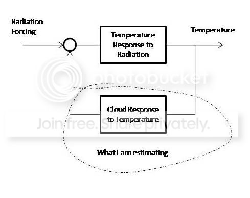
In one of his recent comments Bart posted this diagram of the system he was modelling:

It's a standard feedback system - just two boxes. But to me it raises this query - how can you isolate the box that you want? Electrically, if you look at input-output of box T2, you can't avoid the fact that T1 is in parallel with it. So you's disconnect the box and do the impulse response or whatever out of circuit. It seems to me that weve been trying to do that analysis in circuit, and getting tripped up with causality issues.

August GISS - Very small rise - TempLS map comparison

GISS rose from 0.59°C (Jul) to 0.61°C (Aug). The rise came partly because they adjusted July down by 0.01 0.59°C. TempLS had measured no change (actually down 0.006°C). I'll show the comparison of world distributions below the jump:



Here is the GISS plot of temperature distribution for August 2011:



And here is the TempLS version, using the GISS base years and levels.colors:


This TempLS output suppresses polar plots, mainly because the projection is haywire. I'll produce another of the whole-world versions which should show this.

FFT, impulse response, clouds, GMST

There has been a lot of interest in the thread at CA which started out looking at correlations between a figure that notionally expresses (unreliably) the part of TOA radiant energy flux attributable to clouds and surface temperature. There is a contention, favored by Spencer and Lindzen, that ST may be affecting clouds, which is a kind of feedback, which in fact is spoken of as a forcing.

There's lots to be said about whether these notions are true, but in this post I want to talk about a kind of analysis proposed by commenter Bart at that site.

Instead of looking at correlations, he proposed in effect to find an impulse response function which will transform temperature (T) into that quantity ΔR_cloud (or dR) by convolution:
\[ dR(t) = \int_{-\infty}^\infty h(t-\tau) T(\tau) d\tau\]

You can this of this as being like applying a smoothing filter but it doesn't smooth - it turns T into dR. The basic idea is that Fourier transformation turns that convolution into a product. Then you can work out the FT \(\hat{h}\) from
\[\hat{h} = \hat{dR}/ \hat{T}\]
invert the FT, and it's done. Along the way there are lots of complex variables, but the answer comes out real.

The papers

Discussion has been stirred by a recent paper SB11 by Spencer and Braswell 2011, discussed here,here,here, and a
 response D11 by Dessler. But the CA thread was about an earlier paper D10 by Dessler (discussed here. The links here will lead you to other papers in the series.

The data

The data file is flux.csv here. It covers about 10 years. Col 9 is the surface temp (Hadcrut3), col 5 is TOA flux measured by CERES, and col 8 is a notional clear sky value. The cloud effect dR is got by subtracting col 8 from col 5. Dessler points out that this is biased, because it in effect extrapolates from clear patches of sky to the whole atmosphere, and the air there is much drier than the global average. So there is less wv IR absorption. He used reanalysis data which corrects for this (but may bring other problems).

Causality

The idea of impulse response comes from a known causal relation. You hit a gong with a hammer - you get a response (afterwards). But fitting an impulse response by FFT does not require any kind of causality. You could replace dR by births in Utah.

So convolving with h will pull in temp numbers from the past and from the future. It could well be that past values of dR affect present T - in fact, this is the conventional view. It's not actually clear how to decide, once you've found h (as you always can) what it means.

FFT, truncation and periodicity

This became a subtopic at CA. I've expressed the concept of impulse response with an infinite integral. But there are two dual problems. You can't compute over an infinite range. And you have to have a finite sample width.

While the relation we explore goes on indefinitely, we only see it for a short time. In FT terms, it helps to pretend that we really have indefinite data, but we've multiplied by a gate function to get the window that we see. The reason that it helps is that the gate function multiplication turns up as a convolution in the frequency domain, which explains a lot of things. And you can choose the form of gate function. Instead of a sharp termination, you can taper. This means some loss of data utility, but avoids spurious effects in the medium/high frequency range.

FFT is a way of implementing the discrete Fourier Transform (DFT). This neatly deals with both sampling and range issues but implementing the FT as a Fourier Series. Here's how I think about that.

You're trying to do something about an infinite line in space (denoting time). But you only see a period of 500 km. Suppose you regard it as part of a circle. The Equator is a familiar one. So you put your data on that and sample over longitudes.

But you'll think of this as a line segment, measured by longitude. And you need an IDL (Date Line). You'll probably put this just to one side of the data period.
(This analogy would work better if we started Lon at 0 at the IDL,  ie Lon+180)

Then you say that the rest of the data on the equator is zero(padding). You divide into discrete longitude intervals, say 8192. And you sample frequency by starting with a sinusoid with period the Earth's circumference, and then its 8192 harmonics.

The impulse response will also be expressed on the equator, and will wrap around. And the convolution integral will be evaluated wrapped around as well.

It's a bit harder to think of frequencies as being periodic. We go through the range from a wavelength of 40,000 km down to 5 km. And 5km is about our sampling length. Surely that 5km wave is very different to the 40,000 km and couldn't be adjacent in a periodic measure?

The answer is beats - or strobing. The trig functions are the underlying theory, but numerically all that counts is what is sampled. Those highest frequencies almost match the sampling frequency, but not quite. The difference is what is sampled, and it is indeed a low negative frequency.

The impulse response

Let's now look at the impulse response. The first thing you'll notice is that it's very noisy, and isn't really localised. Why?

You might expect it to be local because for most of its range it produces a zero response on convolution. Zero values would do that.

But in fact it just need to be orthogonal to the T data. That's just one vector in a 8192-dimensional space. h can wriggle as much as it likes, with only that very modest constraint.

So we'll need to smooth it to see anything. Smoothing generally violates that orthogonality, so it won't work exactly as a impulse function afterward. Maybe the smoothing could respect the orthoginality? Yes, more sophisticated filters would help. Here it's just triangular. So here are plots. In terms of the equator notion, I've shifted the date line to the other side of the world from where we have data, and I'm looking at a central window in  the plot. Smoothed on the right with a 10-month triangle filter.




The smoothed version was smoothed across the "date line". The behavious is somewhat different on each side, which I'd like to understand better. So these are the impulse responses that will be used for convolutions.

Bart's h taper.

I don't want to make too much of this, as I don't think it's responsible for any majorly incorrect results. But it doesn't help, and messes up interpretation of the results. In Equator terms, suppose we did have data for 500 km to the E of the IDL. Then Bart said, OK the impulse response doesn't mean anything far away, so we'll taper it off over S America, But his taper continued right around to the IDL. The roll-off was a Hann filter, which is quite good. But the revised smoothed plot now looks like:

Regenerating with convolution

As commenter Steve noted at CA, the test is how well do these work when actually convolved with T

There are some subtleties here in the conventions used with convolve functions. Basically, which way around h is to be used, and taking account of the fact that we are on a circle. R has a convolve function, and you need the options type="circular" and conj=F.

But then, the original unaltered h does give exactly dR. That's not proving anything except that the algebra worked. The smoothed version is rather different, and to me says that we need better smoothing. And the Bart truncation makes a significant difference - probablymore than smoothing.

In these plots, look to the legends for the colors. Because the red reconstructed dR is exact (to plotting accuracy) I've widened the black dR so it doesn't totally disappear under the red.

Regression coefficients

The Dessler-style analysis does regression to say that dR is proportional to T, and the proportionality becomes identified as a feedback factor. Here that is as if the h was compressed into a big spike, and you'd look at the area underneath. That's effectively what Bart is doing when he does another FFT and looks at the zero value. He got -9.4 W/m2/°C. If it weren't for the taper, that FFT is reundant; he could have looked at the f=0 value of the \(\hat(h)\) derived originally. Without the taper, that returns -12.22 W/m2/°C. As he points out, decidedly negative. That's in the direction of the SB and LC interpretations, though it doesn't necessarily contradict Dessler.

But that gives an important clue to what these numbers mean. The data has mean zero. The low frequency end of the FT is actually a moment-generating function. It returns the moments of the data set, and at VLF, that means the first - the regression slope.

So this number -12.22 W/m2/C is actually found by doing time regressions of dR and T over the 10-yr window. If you do this, you get

OLS grad of temp is 0.000412 °C/month
and the grad of dR is -0.005039 W/m2/month
So if you divide the dR slope by the T slope, you get, exactly,
-.005039/.000412= -12.22 W/m2/C

But you'd get such a number from any two series. . It doesn't imply feedback on its own. To do that, you have to have several points showing an association of change in dR with change in T.

Enough for now

There's lots more to say - this is interesting material. I'd like to talk about different ways of dealing with the original data (Hann tapering). I'd like to see what can be said about the mid-range frequencies, where some evidence might be found. Maybe even get into Laplace transforms, which do allow you to take account of causality.

This stuff can generate a huge number of graphs. And I've been dabbling with Javascript tricks to make that more user-friendly. But that's for another day.

Impulse responses and the Spencer/Dessler Cloud models

I've been involved in discussions at this CA thread, which has gone into FFT analysis of the relation between temperature and cloud contribution to TOA energy flux, as discussed a lot re papers from Dessler and Spencer and Braswell.

I should hasten to add that the analysis at CA is based on the use of all CERES data, which Dessler did not do. He gave good reasons for his choice to use reanalysis instead. Consequently, I don't think this alternative approach is telling us anything useful about clouds. However, there is interesting maths.

Commentator Bart there proposed a model in which an impulse function is found by FFT which, when convolved with surface temp (Hadcrut3) will reproduce that "cloud forcing" function, in his notation dR (for δR_cloud). He has produced a lot of Matlab analysis. His contention is that the low frequency behaviour of the impulse response shows strong negative feedback. I don't now agree with that - I think he is looking at very low frequency results which can't be supported by the short period (about 10 years) of data. Furthermore the integral of the impulse response that he cites is the low frequency limit where it becomes just the ratio of the time gradients of the two data sets as determined by OLS regression.

Anyway, I translated his code into R and did some comparison calculations, which I put n a page attached to this blog. I'm now transferring it to this post, in case people want to comment. I'm hoping to write a more detailed analysis soon. The data being used, referred to in the code as flux.csv, is here.



I have converted Bart's matlab code to R - see below. I've only done as far as the impulse response so far.
I'm testing a Hanning window - a cos^2 function which tapers to zero at both ends of the data.

When you FFT a finite set of data, it's as if you did the full set with a gate function. You have to accept low frequency problems with finite data, but the gate adds HF signal as well. A Hanning window tapers much faster in the freq domain, and mitigates this extra problem.

First a check that my R code is getting Bart's result. I've commented out the taper line:





Now after applying the Hanning taper to temp and dR

Update. Steve at CA asked to see if these impulse responses could be convolved with the temp to give dR, which is really what they are for. It's a useful check. In R, you have to use type="circular" and conj=F in the convolve() options. That done, it works. In the plots below, black is the original dR (cloud radiance), red uses the unsmoothed impulse response, and the cyan is the smoothed impulse response. I made the black wider so you can see the red superimposed.

The plot on the right is the same, but smoothed with a 10 month triangle filter. This was done without the Hann tapering of the data. I should clarify that the smoothed impulse response referred to here is the top graph. I have not showed the unsmoothed response - perhaps Bart has. 

Update I've added in dark gold the result of convolving with the taper (w) that Bart used on h. This taper makes h effectively one-sided in time.

Here's the R code. I've tried to follow Bart's notation and steps.
Update - the code originally here deviated in minor ways - I've added fixes

data=read.csv("flux.csv",skip=0);
data[is.na(data)]=0;
temp=data[,9];
dR=data[,5]-data[,8];
N=length(dR);
h=abs(1:N-64.5)/62.5
h[h>1]=1;Ha=cos(h*(pi/2))^2;  #  Hanning Window
temp=temp*Ha; dR=dR*Ha; #  Tapering
dT=1/12;
Nsamp=8192/2;
Npad=Nsamp-N;
X=fft(c(temp,rep(0,Npad)))+1.0e-9;
Y=fft(c(dR,rep(0,Npad)));
h = Re(fft(Y/X,inv=T))/dT/Nsamp;
Nc=Nsamp/8;
w=c(rep(1,Nc),(1-cos(pi*(1:Nc-1)/(Nc-1)/2)),rep(0,Nsamp-6*Nc))
hw=h*w;
f1=c(1:15,15:1); f1=f1/sum(f1);
hs=filter(h,f1)
t=(0:599)*dT
png("impresHanning.png");
plot(t,hs[1:600],type="l",ylab="Impulse Response W/m2/C/yr",xlab="Years",main="Cloud-Temperature System Smoothed Impulse Response/Hanning")
dev.off()

Late final extra

Carrick asked to see the mag plot of h. I've followed Bart's scheme, with log axes. It's weighted towards low frequencies. This h has neither my Hann taper of data nor Bart's h truncation. Mag and phase:

August GMST - TempLS no change

This is the second month of running a TempLS analysis ahead of the major indices, and coincidentally with the same result. August's mean land/sea temperature anomaly came out the same as July - 0.45°C, relative to the 1961-1990 base period. The data and plots are at the latest ice and temperature data page.

Below is the graph (lat/lon) of temperature distribution for August, using GISS colors, levels and base period



And here, from that data page, is the plot of the last four months: