The GISS V4 land/ocean temperature anomaly was 0.74°C in April 2021, down from 0.88°C in March. This is similar to the 0.165°C decrease (now 0.134) reported for TempLS. Jim Hansen's report is here.
As usual here, I will compare the GISS and earlier TempLS plots below the jump.
Friday, May 14, 2021
Wednesday, May 5, 2021
April global surface TempLS down 0.165°C from March.
The TempLS mesh anomaly (1961-90 base) was 0.608°C in April, down from 0.773°C in March. That takes away much of the rise in March, and goes back to about the level in Dec/Jan, though warmer than February. It was the coolest April since 2013. The NCEP/NCAR reanalysis base index did not rise as much in March, and so did not fall in April, rising just 0.016°C. Again, April was about the level of Dec/Jan.
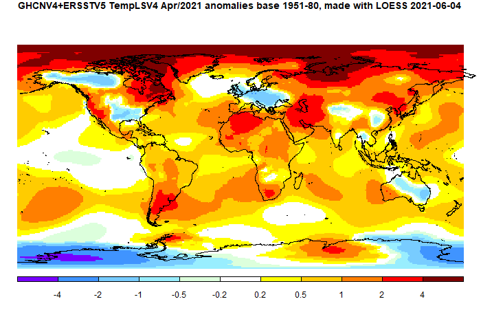
Many Moyhu readers will have experienced the cold patches, which were in Eastern US (also Alaska and NW Canada), Europe and most of Australia. There was also a cold band through Afghanistan/China. N Africa, S America, NE Canada and NW Siberia (and much of Arctic) were warm; Antarctica was cold.
Here is the temperature map, using the LOESS-based map of anomalies.
 As always, the 3D globe map gives better detail.
Many Moyhu readers will have experienced the cold patches, which were in Eastern US (also Alaska and NW Canada), Europe and most of Australia. There was also a cold band through Afghanistan/China. N Africa, S America, NE Canada and NW Siberia (and much of Arctic) were warm; Antarctica was cold.
Here is the temperature map, using the LOESS-based map of anomalies.
As always, the 3D globe map gives better detail.Monday, May 3, 2021
CMIP6 comparing TOS with observed SST, and blended TOS/TAS with GISSlo
This post is a sequel to my recent post, which reviewed a claim by Dr Roy Spencer that the new round of CMIP6 modelling gave warming in the 1979-2020 period twice what was observed. One of the issues was that he had used TAS (surface air) instead of TOS (sea surface) to compare with observed SST. The data source he used, KNMI, does not at present have CMIP6 TOS results, so nor did I.
However, Gavin Schmidt noted that there was a new repository at University of Melbourne which had more results available, including TOS. This is a useful repository in which a lot of averaging is pre-done. The supporting paper by Nicholls et al is here. And indeed, it does have currently TOS results from 13 models, and also a wider range of TAS.
This makes it possible for me to update the plots of the last post, which used TAS restricted to ocean (following Roy), which I adjusted using the difference trend from CMIP5. But it also makes it possible to calculate the correct blend of TOS/TAS to match the commonly quoted land/ocean observed indices.
In 2015, Cowtan, Hausfather et al published a paper in which the noted that comparisons of modelled and observed frequently compared modelled TAS with observed land/ocean, which is not like with like. They created a blended CMIP5 set using TAS on land and TOS at sea. It makes a considerable difference. I do something similar here, but for the rather limited set posted so far.
As before, the CanESM results, of which there are two, are clearly the most rapidly warming. If you exclude them, the observed is in the centre of the modelled range. For comparison, here is my previous plot in which I showed TAS with a trend adjustment from CMIP5 TAS/TOS:
However, Gavin Schmidt noted that there was a new repository at University of Melbourne which had more results available, including TOS. This is a useful repository in which a lot of averaging is pre-done. The supporting paper by Nicholls et al is here. And indeed, it does have currently TOS results from 13 models, and also a wider range of TAS.
This makes it possible for me to update the plots of the last post, which used TAS restricted to ocean (following Roy), which I adjusted using the difference trend from CMIP5. But it also makes it possible to calculate the correct blend of TOS/TAS to match the commonly quoted land/ocean observed indices.
In 2015, Cowtan, Hausfather et al published a paper in which the noted that comparisons of modelled and observed frequently compared modelled TAS with observed land/ocean, which is not like with like. They created a blended CMIP5 set using TAS on land and TOS at sea. It makes a considerable difference. I do something similar here, but for the rather limited set posted so far.
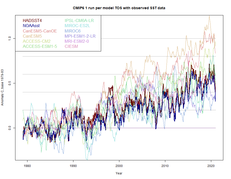
CMIP6 and TOS
There are 10 models that provide TOS results, and this time I plot just the first for each model type. They are normalised so that the 1979-1983 average is zero, for each month. The result isAs before, the CanESM results, of which there are two, are clearly the most rapidly warming. If you exclude them, the observed is in the centre of the modelled range. For comparison, here is my previous plot in which I showed TAS with a trend adjustment from CMIP5 TAS/TOS:
Blending TOS/TAS to compare with observed land/ocean.
As said above, CMIP TAS results are often compared with modelled land/ocean, with much the same problems as in Roy Spencer's usage. Cowtan et al (2015) derived a combined TOS/TAS for CMIP5. They did a cell by cell calculation of the blend. I think it is arithmetically equivalent to use the posted land average TAS with TOS, provided the weighted combination uses the same land/sea mask to calculate areas as it did to average the temperature subsets. In this case, I used the areas that were provided with the TAS/TOS data (in the header), so I hope that is true. If not, it won't make a big difference. The land fraction was 0.287.Update 5 May 2021. I made an error in the initial post; I used the wrong column blended with sea TAS instead of land TAS. It makes a considerable difference, although the relative position of GISS is as originally described. The old plot is <a href="https://s3-us-west-1.amazonaws.com/www.moyhu.org/2021/05/blend1.png">here</a>. The zip file linked below has been updated.
I blended always TOS/TAS runs that had the same variant number, although that common value may vary from model to model. Again, I chose one blend from each model, and compared with GISS land/ocean:
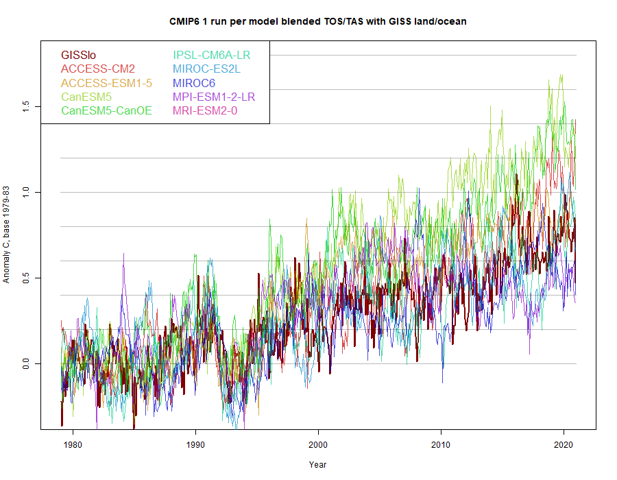
Again, the CanESM results warm fastest, and GISS sits on the warm side of the other results. For comparison, I plotted what would happen using TAS global alone, as is often done
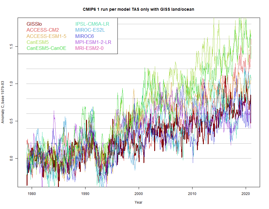
Even excluding CanESM, it now appears that modelled results run warmer than GISS. They are also a lot more variable. It is important to compare with the blend.
I blended always TOS/TAS runs that had the same variant number, although that common value may vary from model to model. Again, I chose one blend from each model, and compared with GISS land/ocean:
Again, the CanESM results warm fastest, and GISS sits on the warm side of the other results. For comparison, I plotted what would happen using TAS global alone, as is often done
Even excluding CanESM, it now appears that modelled results run warmer than GISS. They are also a lot more variable. It is important to compare with the blend.
Data posted
I have posted a zipped csv file here, with blends for 102 runs from 1850 to 2101, with a readme file and some headers. Update 5 May 2021. I made an error in the initial post, see above. The file has been updated.
Subscribe to:
Posts (Atom)


