Here is the GISS spatial distribution:

and the TempLS spherical harmonics LS fit:

Past months:
| Sep | GISS Sep 11 - down 0.13°C |
| Aug | August GISS - Very small rise - TempLS map compari... |
| July | Comparisons of TempLS with reader MP's July 2011 ... |


| Sep | GISS Sep 11 - down 0.13°C |
| Aug | August GISS - Very small rise - TempLS map compari... |
| July | Comparisons of TempLS with reader MP's July 2011 ... |
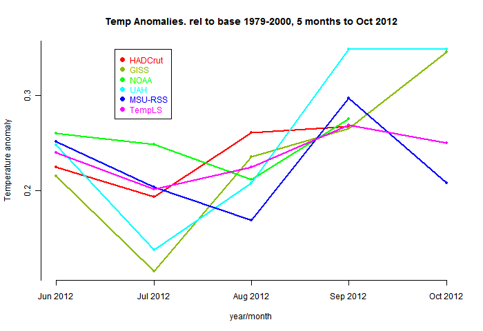
Hmm, what does it mean when the satellite temps head in the opposite direction to the surface temps?
ReplyDeleteIf the global temperatures are being supported by polar warmth, then HADCrut is going to show cooling.
Kevin C
KevinC: Hmm, what does it mean when the satellite temps head in the opposite direction to the surface temps?
ReplyDeleteWell here's my view since I haven't seen any takers on that question:
In order to compare month-to-month time-series, there are several criteria that the signals being compared must satisfy. One is that they are phase linear at that frequency rate (and that the two signals are in phase..)
The fact they are different is likely at least partly related to the difference in what they are measuring (surface air temperature inside the atmospheric boundary layer versus well-mixed tropospheric temperature), partly due to different systematic errors partly due to noise sources (including systematic error introduced by the averaging process).
If you really want a metric for comparison, look either at the coherence between two series, or the power spectral density (PSD) within a single series. The "real" global mean temperature should have a seasonal component in it (even after anomalization, and I can expand on why I believe that to be true), which means there should be an annual component in the PSD as well as sub-annual harmonics.
A comparison of HACRUT, GISTEMP and UAH actually reveals that UAH may have over-corrected for seasonal effect (there are notches in the UAH PSD at these frequency components), meaning that UAH is essentially worthless in looking at sub-annual variation. The other series generally don't agree that well on sub-annual too. It depends on the details of how well you did the annual average for how much of the seasonal component survives the averaging. Done entirely wrong, you end up just smearing out the spectral peaks, and again just end up with garbage for sub-annual variability.
Sorry if this is a bit terse, I can expand on this if what I am saying is unclear.
Carrick,
ReplyDeleteThanks. There is also (I believe) a view that satellite troposphere temperatures are a leading indicator of GMST change. I've been trying to track down my source for that belief.
Thanks both! The annual cycle stuff is interesting. I've just established that a residual annual cycle is the primary remaining difference between my recreation of CRUTEM3 and the real thing - presumably as a result of my 'improved' station alignment technique (a quick-and-dirty iterative approximation to Nick's). I can see that could be a factor, and it's one that is easily testable.
ReplyDeleteIf tropo temps are a leading indicator of GMST, then that should also be testable with a lag analysis. So many interesting calculations to do...
Kevin C
Kevin C: I've just established that a residual annual cycle is the primary remaining difference between my recreation of CRUTEM3 and the real thing - presumably as a result of my 'improved' station alignment technique (a quick-and-dirty iterative approximation to Nick's).
ReplyDeleteIt's my belief that this technique (which actually originated with RomanM as I understand it) reduces the amount of "spectral smearing" associated with anomalization. I believe all of the "traditional"/"professional" reconstructions suffer from this spectral smearing to different extents.
In terms of lag differences, if you know that the data are getting highly filtered, you need to be careful that there isn't a phase lag introduced by the filtering—and if the filters are different between different algorithms, the same frequency component can have different group delays associated with the roll-off of the filter—and you could end up with different amplitudes and different lags associated with high frequency phenomena between different reconstructions.
I implemented a method of station combination which originally I thought was a version of Tamino's but I'm not sure if it is different or not. I manually did this in excel way back at the start of 2010 and have since been more interested in using Nick's or Tamino's methods using the RGHCN Processor (Mosher) but I was wondering how the method sounds mathematically. I'm still not 100% sure how I could summarize it in a formula but anyways...
ReplyDeleteThe method is as follows:
Average all station data available for each month into a simple average. Calculate the average for the simple average and each active station for the overlapping months (between the simple average of all and the individual station).
Adjust the values of each station by the offset calculated between the individual station and the overlapping period of the simple average to "align" stations. This is done simultaneously for all stations.
I sum the offsets and iteratively repeat until the sum of the offsets is less than 0.009 (Arbitrary).
My result on a test region gives virtually the same as yours on the annual basis. Obviously weights and spatial coverage aren't included but have you guys got any thoughts on this method, particularly about the math?
Robert,
ReplyDelete"Calculate the average for the simple average and each active station for the overlapping months (between the simple average of all and the individual station)."
I got lost at this stage. Could you try with latex? Just $_$ ...$_$ or \_(..|_) (remove _ ) invokes it. Or I often just use suffixes indicated with _, so I'd write your first proposition as
U_my = Σ T_smy/N_my
where smy are station, month and year, N_my total stations in each month etc.
I'm guessing Robert is describing the same approach I'm using. The problem is as follows:
ReplyDeleteThe station temps t are given by a combination of global temp T, local offset d (by month), and noise e:
$$ t_{s,y,m} = T_{y,m} + d_{s,m} + e_{s,y,m} $$
Then the global temp is calculated from the station temps. I guess Robert like me is using a gridded method, but it comes down to:
$$ T_{y,m} = ( \sum_{s} w_{s,y,m} ( t_{s,y,m}-d{s,m} ) ) / ( \sum_{s} w_{s,y,m} )$$
where hopefully the e's get averaged away.
As I understand it, you solve these simulteneously by LS, along with a few extra eqns which effectively set the baseline.
What I'm doing is first estimating the d's to align stations on 1950-1980 (only works for long dunning stations, to get an initial T, then iteratively updating d's then T until convergence. (Well, just 3 cycles in my case). Which hould give an approximation to your method, although less formal about how the errors get distributed.
I think Robert is doing the same, apart from starting with T. Is that right?
Kevin C
p.s. LaTeX doesn't work in preview, hope I got it right. If not, no doubt you can read the LaTeX straight off.
Thanks, Kevin, that helps. Here's my take.
ReplyDeleteI like to use the summation convention with padding arrays filled with 1's. So I'd write the weighted set of residuals as
$$W_{(sym)}R_{sym},\_\_R_{sym}=(t_{sym}-I_yd_{sm}-I_sT_{ym})$$
No summation so far, (the W indices are exempt) but then you try to solve the system:
$$ I_sW_{(sym)}R_{sym}=W_{(sym)}(I_st_{sym}-I_sI_yd_{sm}-I_sI_sT_{ym})=0$$
$$J_y(I_st_{sym}-I_sI_yd_{sm})=0$$
by iteration, where \(J_y\) has 1's from 1951-80, 0 elsewhere. The second is the matching equation.
Well there would be enough equations to match unknowns if the second equation was non-trivial for all stations, but it isn't, so the process may not converge completely.
In fact the first equation you have is what you get by minimising the sum of squares
$$W_{(sym)}R_{sym}^2$$ wrt T only - ie differentiate wrt T. The LS equation minimising wrt d is:
$$ I_yW_{(sym)}R_{sym}=0$$
similar to yours, but without gaps for series with no 1951-80 overlap.
Apologies, I think that second eqn should be
ReplyDelete$$J_y(t_{sym}-I_yd_{sm})=0$$
Oh, yes, that makes sense.
ReplyDeleteI missed out a couple of details. Only the first cycle is against 1951-1980 - essentally against a T(y,m) which is zero on that period and non-existant outside. However, the first cycle gives us an estimate of T covering the whole period. On subsequent cycles, all stations with 15 months of data ever are used. (Even the 15 month criterion could be relaxed, but I kept it for consistency with CRU.) That increases the available station months of data by about 20%.
Also, as you spotted, the calculation can drift off from the baseline without a set of 12 extra equations. I've seen this happening and added a third step where I renormalise T(y,m) for each of the 12 months on the baseline period. This is the only role the baseline period plays after the first cycle.
I've now achieved what I was aiming for - diagnosing the divergence between CRUTEM3 and BEST. Apart from the NH/SH weighting, which BEST already took into account, the biggest remaining difference is actually not due to the poor coverage, but due to the lack of a land mask - particularly bad for CRU's big 5deg cells. Just adding a term weighting each cell by the proportion of land in that cell brings CRUTEM3 into a good decadal agreement with BEST (even better with NOAA). I've passed this on to the BEST team:
[GRAPH HERE]
The trend within the last decade however is strongly influenced by the lack of infilling.
Kevin C
Kevin C - thanks for the graph. It will be interesting to see how BEST responds, and how this all ends up once they've finished the globe.
ReplyDeleteKevin,
ReplyDeleteI was thinking more about your method. It doesn't minimise SS residuals, but probably gets close. And your system is triangular, so no matrices to invert.
The LS method with conjugate gradient iteration also converges very fast. The arithmetic needed for each step is comparable. And that's without preconditioning.
I think what you have is a very good preconditioner. You could use the LS equations as the target of your iteration. That is, compute the sum of weighted iterations over years and use that (with - sign) as the right hand side of your second equation on iteration.
hey all,
ReplyDeleteI will comment later on regarding the math with my method. Having taken a bit of time to read over some stuff I feel that essentially it is Tamino's method but with the computation of offsets for stations being calculated simultaneously against the regional average rather than one at a time which I thought his method does. He also sets the first reference station to zero.
It might take me a bit to digest some of the maths. It is afterall not my subject area.
Nick: Yes. It's time to put the full LS calc on my things to do list, to see how much the final result differs from the 'preconditioned' one. I'll need to learn to use the equation solvers in SciPy. Or just learn R, which I have to do anyway, given that I'm teaching it in a couple of years. I'm mostly being driven by results at the moment, so still taking the easiest rather than best route to an answer.
ReplyDeleteRobert: Oh, so I read my method into your post, rather than interpreting what you were saying. Confirmation bias at work!
Kevin C