The essential steps are a least squares fitting of normals for each location and month, which are then subtracted from the observed temperatures to create station anomalies. These are then spatially integrated to provide a global average. The main providers who also to this do not generally post their local anomalies, but I have long wanted to do so. I have been discouraged by the size of the files, but I have recently been looking at getting better compression, with good results, so I will now post them.
The download file
The program is written in R, and so I post the data as a R data file. The main reason is that I store the data as a very big matrix. The file to download is here. It is a file of about 6.9 MBytes, and contains:- A matrix of 10989 locations x 1428 months, being months from Jan 1900 to Sep 2018. The entries are anomalies to 1 decimal place normalised to a base of 1961-90.
- A 10989x12 array of monthly normals. These are not actually the averages for those years, but are least squares fitted and then normalised so the global average of anomalies comes to zero over those years. Details here. You can of course regenerate the original temperature data by adding the anomalies to the appropriate normals.
- A set of 1428 global monthly global averages.
- An inventory of locations. The first 7280 are from the GHCN inventory, and give latitude, longitude and names. The rest are a subset of the 2x2° ERSST grid - the selection is explained here.
- A program to unpack it all, called unpack()
packed$unpack(packed)
will cause a regular R list with the components described above to appear in your directory.
Compression issues and entropy
The back-story to the compression issue is this. I found that when I made and saved (with gzip) an ordinary R list with just the anomalies, it was a 77 MByte file. R allows various compression options, but the best I could do was 52 MB, using "zx" at level 9. I could get some further improvement using R integer type, but that is a bit tricky, since R only supports 32 bit integers, and anyway it didn't help much. That is really quite bad, because there are 15.7 million anomalies, which can be set as integers of up to a few hundred. And it is using, with gzip, about 35 bits per number. I also tried netCDF via ncdf4, using the data type "short" which sounded promising, and compression level 9. But that still came ot 47 MB.So I started looking at the structure of the data to see what was possible. There must be something, because the original GHCN files as gzipped ascii are about 12.7 MB, expanding to about 52 MB. The first thing to do is calculate the entropy, or Shannon information, using the formula
H = sum - pi log2(pi)
where p is the frequency of occurrence of each anomaly value. If I do that for the whole matrix, I get 4.51 bits per entry. That is, it should be possible to store the matrix in
1.57e+7 * 4.51/8 = 8.85 MB
But about 1/3 of the data are NA, mostly reflecting missing years, and this distorts the matter somewhat. There are 1.0e+7 actual numbers, and for these the entropy is 5.59 bits per entry. IOW, with NA's removed, about 7 MB should be needed.
That is a lot less than we are getting. The entropy is based on the assumption that all we know is the distribution. But there is also internal structure, autocorrelation, which could be used to predict and so lower the entropy. This should show up if we store differences.
That can be done in two ways. I looked first at time correlation, so differencing along rows. That reduced the entropy to only 5.51 (from 5.59). More interesting is differencing columns. GHCN does a fairly good job of listing stations with nearby stations close in the list, so this in effect uses a near station as a predictor. So differencing along columns reduces the entropy to 4.87 bits/entry, which is promising.
More thoughts on entropy
Entropy here is related to information, which sounds like a good thing. It's often equated to disorder, which sounds bad. In its disorder guise, it is famously hard to get rid of. In this application, we can say that we get rid of it when we decide to store numbers, and the amount of storage is the cost. So the strategic idea is to make sure every number stored carries with it as much entropy as possible. IOW, it should be as unpredictable as possible. I sought to show this with the twelve coin problem. That is considered difficult, but is easily solved if you ensure every weighing has a maximally uncertain outcome.I'll describe below a bisection scheme. Whenever you divide, you have to store data to show how you did it, which is a significant cost. For dividing into two groups, the natural storage is a string of bits, one for each datum. So why bisection? It maximises the uncertainty. Without other information, each bit has an equal chance of being 1 or 0.
I should mention here too that, while probability ideas are useful, it is actually a deterministic problem. We want to find a minimal set of numbers which will describe another known set of numbers.
Radix compression
The main compression tool is to pack several of these anomalies into a 32 or 64 bit integer. There are just 360 numbers that occur, so if I list them with indices 0..359, I can treat 3 as digits of a base 360 number. 360^3 is about 4.66e+7, which can easily be expressed as a 32 bit integer. So each number is then using about 10.66 bits.One could stop there. But I wanted to see how close to theoretical I could get. I'll put details below the jump, but the next step is to try to separate the more common occurrences. I list the numbers in decreasing order of occurrence, and see how many of the most common ones make up half the total. there were 11. So I use up one bit per number to mark the dividion into two groups, either in or out of that 11. So I have spent a bit, but now that 5 million (of the 10m) can be indexed to that set and expressed to the base 11. We can fit 9 of those into an unsigned 32 bit integer. So although the other set, with 349 numbers, will stil require the same space for each, half have gone from 10.3 bit's each to 3.55 bits each. So we're ahead, even after using one bit for indexing.
Continuing with bisection
We can continue to bisect the larger set. There will again be a penalty of one bit per data point, in that smaller set. Since it halves each time, the penalty is capped at 2 bits overall for the data. The following diagram illustrates how it works. I have assumed that the anomalies, rendered as integers, are normally distributed, with the histogram in faint grey. The sigmoid is the cumulative sum of the histogram. So in the first step, the red block is chosen (it should align with the steps). The y axis shows the fraction of all data that it includes (about half). The x axis shows the range, in integer steps. So there are about 11 integers. That can be represented with a little over 3 bits per point.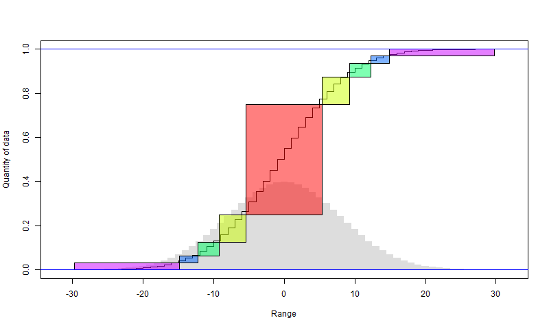
The yellow comes from a similar subdivision of the remainder. It includes a quarter of the total data, and also has a range of about 11 values (it doesn't matter that they are not consecutive)
And so on. I have shown in purple what remains after four subdivisions. It has only 1/16 of the data, but a range that is maybe not much less than the original range. So that may need 10 bits or so per element, but for the rest, they are expressed with about 3 bits (3.6). So instead of 10 bits originally, we have
2 bits used for marking, + 15/16 * 3.6 bits used for data + 1/16*10 for remainder
which is about 6 bits. Further subdivision would get it down toward 5.6
Update I have plotted a budget of how it actually worked out, for the points with NA removed and differenced as described next. . The Y axis is the number of 32 bit integers stored per data point. Default would be 1, and I have shown in light blue the level that we would get with simple packing. The X-axis is number of data, so the area is the total integers packed. The other columns are the results of the bisection. The red is the integers actually packed for the values in that set, and the green is the number of bits to mark the divisions, attributed between the set in each division. There were six divisions.
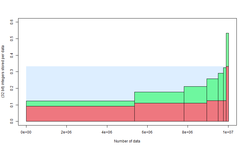
Although this suggests that dividing beyond 6 is not worthwhile, it is, because it still adds just one bit while substantially reducing half the remaining red.
Differencing
As said earlier, there is a significant saving if the data is differenced in columns - ie in spatial order. In practice, I just difference the whole set, in column order. The bottom of one column doesn't predict the top of the next, but it only requires that we can predict well on average.Strategy
You can think of the algorithm as successively storing groups of numbers which will allow reconstruction until there are none left. First a binary list for the first division is stored (in 32 bit integers), then numbers for the first subgroup, and so forth. The strategy is to make sure each has maximum entropy. Otherwise it would be marked for further compression.The halving maximises entropy of the binary lists. And the subgroups that are stored, from the centre out, are OK to store, because there is little variation in the occurrence of their values. The first is from the top of the distribution, and although the smaller rectangles are from regions of greater slope in the histogram, they are short intervals and the difference isn't worth chasing.
Missing values
I mentioned that about a third of the data, when arranged in this big matrix, are missing. The compression I have described actually does not require the data to be even integers, let alone consecutive, so the NA's could be treated as just another data point. However, I treat them separately for a reason. There is a penalty again of one bit set aside to mark the NA locations. But this time, that can be compressed. The reason is that in time, NA's are highly aggregated. Whether you got a reading this month is well predicted by last month. So the bit stream can be differenced, and there will be relatively few non-zero values. But that requires differencing by rows rather than columns, hence the desirability of separate treatment.After differencing, the range is only 3 (-1,0,1), so the bisection scheme described above won't get far. So it is best to first use the radix compression. To base three, the numbers can be packed 20 at a time into 32 bit integers. And the zeroes are so prevalent that even those aggregated numbers are zero more than half the time. So even the first stage of the bisection process is very effective, since it reduced the data by half, and the smaller set, being only zero, needs no bits to distinguish the data. Overall, the upshot is a factor of compression of about 5. IOW, it costs only about 0.2 bits per data point to rempve NA's and reduce the data by 33%.
Summary
I began with an array providing for 15 million anomalies, of which 5 million were missing. Conventional R storage, including compression, used about 32 bits per datum, not much better than 32 bit integers. Simple radix packing, 3 to a 32 bit integer, gives a factor of 3 improvement, to about 10.7 bits/datum. But analysis of entropy says only about 5.6 bits are needed.A bisection scheme successively removing the numbers occurring most frequently that account for half the remaining data, recovers almost all of that difference. A further improvement is made by differencing by columns (spatially). Missing values can be treated separately in a way that exploits their tendency to run in consecutive blocks in time.
Update I should summarize the final compression numbers. The compressed file with inventory and normals was 6.944 MB. But with the anomalies only, it is 6.619 MB, which is about 3.37 bits/matrix element. It beats the theoretical because it made additional use of differencing, exploiting the spatial autocorrelation, and efficiently dealt with NA's. Per actual number in the data, it is about 5.3 bits/number.