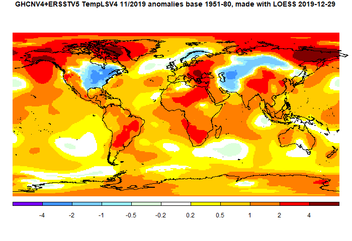
The GISS V4 land/ocean temperature anomaly stayed at 1.02°C in November, same as October. It compared with a 0.063deg;C fall in TempLS V4 mesh (latest figures). GISS also had 2019 as second-warmest November after 2015.
Updating of GHCN V4 this month is fitful, so this figure may change. I see that BEST has delayed publishing November's result.
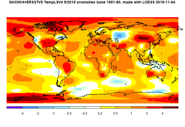
The overall pattern was similar to that in TempLS. Cool band through Central Asia into Siberia. Warm just about everywhere else, especially Arctic.
As usual here, I will compare the GISS and earlier TempLS plots below the jump.
Tuesday, December 17, 2019
Saturday, December 14, 2019
November global surface TempLS down 0.063°C from October.
The TempLS mesh anomaly (1961-90 base) was 0.824deg;C in November vs 0.887°C in October. This was similar to the 0.067°C fall in the NCEP/NCAR reanalysis base index. This makes it the second warmest November in the record, after the El Niño 2015. So it almost certain that 2019 will be the second warmest year after 2016 (currently averaging 0.811°C vs 0.855 for 2016). However, so far December has been exceptionally warm, which could bring 2019 even closer.
As I posted yesterday, GHCN data was delayed this month. The file dates posted remained at 6 Dec until just recently, when one dated 12 Dec appeared. It still seems a little lightweight for the date, but it gives me more than my target minimum of 12000 total stations or posting. Actually FWIW waiting didn't make much difference; the earlier file gave an average of 0.828°C.
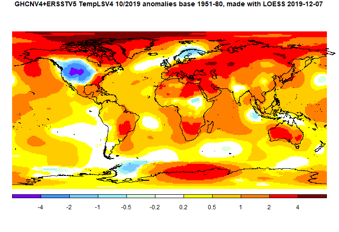
The pattern echoed features of the recent months. Once again a cold spot in N America, this time east of the Rockies, and also a hot spot over Alaska/NW. This extends to very warm in NE Siberia and the Canadian Arctic islands. Warm in Arctic generally, and a band from E Europe right down through Africa, A cold band in central Asia.
Here is the temperature map, using the LOESS-based map of anomalies.
 As always, the 3D globe map gives better detail.
As I posted yesterday, GHCN data was delayed this month. The file dates posted remained at 6 Dec until just recently, when one dated 12 Dec appeared. It still seems a little lightweight for the date, but it gives me more than my target minimum of 12000 total stations or posting. Actually FWIW waiting didn't make much difference; the earlier file gave an average of 0.828°C.
The pattern echoed features of the recent months. Once again a cold spot in N America, this time east of the Rockies, and also a hot spot over Alaska/NW. This extends to very warm in NE Siberia and the Canadian Arctic islands. Warm in Arctic generally, and a band from E Europe right down through Africa, A cold band in central Asia.
Here is the temperature map, using the LOESS-based map of anomalies.
As always, the 3D globe map gives better detail.Friday, December 13, 2019
November global surface temperatures delayed.
The usual TempLS calculation of global temperature is awaiting new posting of GHCN V4 surface land data from NOAA. The last update was on 7 December, although even that seemed to be the same as the day before.
The data is currently missing China, Kazakhstan and Mexico. FWIW it shows a drop from October of about 0.06°C. I'll post as soon as new data appears. I usually wait until we have 12000 or more stations (including SST) - currently 10284.
The data is currently missing China, Kazakhstan and Mexico. FWIW it shows a drop from October of about 0.06°C. I'll post as soon as new data appears. I usually wait until we have 12000 or more stations (including SST) - currently 10284.
Tuesday, December 3, 2019
November global surface reanalysis down 0.067°C from October.
The Moyhu NCEP/NCAR index fell from 0.475°C in October to 0.408°C in November, on a 1994-2013 anomaly base. That brings it back to about the level of the previous month, but continues the relatively stable warm period since May.
Most of North America was cool, except toward Alaska. far W Europe and most of Russia/Iran also cool. Central Europe was warm, elsewhere mixed. NE Pacific and Greenland were warm.

Most of North America was cool, except toward Alaska. far W Europe and most of Russia/Iran also cool. Central Europe was warm, elsewhere mixed. NE Pacific and Greenland were warm.
Saturday, November 23, 2019
A good faith article by a recovering sceptic, but needs care with sources.
There is an interesting article in Reason by Ron Bailey, titled "What Climate Science Tells Us About Temperature Trends" (h/t Judith Curry). It is lukewarmish, but, as it's author notes, that is movement from a more sceptical view. It covers a range of issues.
His history shows up, though, in prominence given to sceptic sources that are not necessarily in such good faith. True, he seems to reach a balance, but needs to be more sceptical of scepticism. An example is this:
"A recent example is the June 2019 claim by geologist Tony Heller, who runs the contrarian website Real Climate Science, that he had identified "yet another round of spectacular data tampering by NASA and NOAA. Cooling the past and warming the present." Heller focused particularly on the adjustments made to NASA Goddard Institute for Space Studies (GISS) global land surface temperature trends. "
He concludes that "Adjustments that overall reduce the amount of warming seen in the past suggest that climatologists are not fiddling with temperature data in order to create or exaggerate global warming" so he wasn't convinced by Heller's case. But as I noted here, that source should be completely rejected. It compares one dataset (a land average) in 2017 with something different (Ts, a land/ocean average based on land data) in 2019 and claims the difference is due to "tampering". Although I raised that at the source, no correction or retraction was ever made, and so it still pollutes the discourse.
A different kind of example is the undue prominence accorded to Christy, and Michaels and Rossiter. He does give the counter arguments, and seems to favor those counters. Since the weighting he gives to those sources probably reflects the orientation of his audience, that may in the end be a good thing, but I hope we will get to a state where these recede to their rightful place.
His conclusion is:
"Continued economic growth and technological progress would surely help future generations to handle many—even most—of the problems caused by climate change. At the same time, the speed and severity at which the earth now appears to be warming makes the wait-and-see approach increasingly risky. Will climate change be apocalyptic? Probably not, but the possibility is not zero. So just how lucky do you feel? Frankly, after reviewing recent scientific evidence, I'm not feeling nearly as lucky as I once did."
Some might see that as still overrating his luck, but it is an article worth reading.
Saturday, November 16, 2019
GISS October global up 0.12°C from September.
The GISS V4 land/ocean temperature anomaly stayed at 1.04°C in October, up from 0.92°C September. It compared with a 0.116deg;C rise in TempLS V4 mesh (latest figures). GISS also had 2019 as second-warmest October after 2015.
The overall pattern was similar to that in TempLS. Prominent cold spot in US W of Mississippi (and adjacent Canada). Warm just about everywhere else (but not Scandinavia).
As usual here, I will compare the GISS and earlier TempLS plots below the jump.
The overall pattern was similar to that in TempLS. Prominent cold spot in US W of Mississippi (and adjacent Canada). Warm just about everywhere else (but not Scandinavia).
As usual here, I will compare the GISS and earlier TempLS plots below the jump.
Friday, November 8, 2019
Structure and implementation of methods for averaging surface temperature.
I have been writing about various methods for calculating the average surface temperature anomaly. The mathematical task is basically surface integration of a function determined by sampling at measurement points, followed by fitting offsets to determine anomalies. I'd like to write here about the structure and implementation of those integration calculations.
The basic process for that integration is to match the data to a locally smooth function which can be integrated analytically. That function S(x) is usually expressed as a linear combination of basis functions Bᵢ(x), where x are surface coordinates
using a summation convention. This post draws on this post from last April, where I describe use of the summation convention and also processes for handling sparse matrices (most entries zero), which I'll say a lot about here. The summation convention says that when you see an index repeated, as here, it is as if there were also a summation sign over the range of that index.
The fitting process is usually least squares; minimise over coefficients b:
where the yj are the data points, say monthly temperature anomalies, at points xj) and K is some kernel matrix (positive definite, usually diagonal).
This all sounds a lot more complicated than just calculating grid averages, which is the most common technique. I'd like to fit those into this framework; there will be simplifications there.
Minimising (2) by differentiating wrt b gives
where H is the matrix Bᵢ(xj)), Hw is the matrix Bᵢ(xj))Kjk and HwH = Hw⊗H* (* is transpose and ⊗ is matrix multiplication). So Eq (4) is a conventional regression equation for the fitting coefficients b. The final step in calculating the integral as
A = bᵢaᵢ
where aᵢ are the integrals of the functions Bᵢ(x), or
The potentially big operations here are the multiplication of the data values y by the sparse matrix Hw, and then by the inverse of HwH. However, there are some simplifications. The matrix K is the identity or a diagonal matrix. For the grid method and mesh method (the early staple methods of TempLS), HwH turns out to be a diagonal matrix, so inversion is trivial. Otherwise it is positive definite, so a conjugate gradient iterative method can be used, which is in effect the direct minimisation of the quadratic in Eq (2). That requires only a series of multiplication s of vectors by HwH, so this product need not be calculated, but left as its factors.
I'll now look at the specific methods and how they appear in this framework.
The matrix H has a row for each cell and a column for each data point. It is zero except for a 1 where data point j is in cell i. The product HwH is just a diagonal matrix with a row for each cell, and the diagonal entry is the total number of data points in the cell (which may be 0). So that reduces to saying that the coefficient b for each cell is just the average of data in the cell. It is indeterminate if no data, but if such cells are omitted, the value would be unchanged if the cells were assigned the value of the average of the others.
Multiplying H by vector y is a sparse operation, which may need some care to perform efficiently.
For a long time I used SH fits, calculating the b coefficients as above, for graphic shade plots of the continuum field. But some other advanced methods provide their own fitted functions.
I described here a rather ad hoc method for iteratively estimating empty cells from neighbors with data, which worked quote well. But the matrix formulation above gives a more scientific way of doing this. You can write a matrix which expresses a requirement that each cell should have the average values of its neighbors. For example, a rectangular grid might have, for each cell, the requirement that 4 times its value - the values of the four neighbors is zero. You can make a (sparse symmetric) matrix L out of these relations, which will have the same dimension as HwH. It has a rank deficiency of 1, since any constant will satisfy it.
Now the grid method gave an HwH which was diagonal, with rows of zeroes corresponding to empty cells, preventing inversion. If you form HwH + εL, that fixes the singularity, and on solving does enforce that the empty cells have the value of the average of the neighbors, even if they are also empty. In effect, it fills with Laplace equation using known cell averages as boundaries. You can use a more exact implementation of the Laplacian than the simple average, but it won't make much difference.
There is a little more to it. I said L would be sparse symmetric, but that involves adding mirror numbers into rows where the cell averages are known. This will have the effect of smoothing, depending on how large ε is. You can make ε very small, but then that leaves the combination ill-conditioned, which slows the iterative solution process. For the purposes of integration, it doesn't hurt to allow a degree of smoothing. But you can counter it by going back and overwriting known cells with the original values.
I said above that, because HwH inversion is done by conjugate gradients, you don't need to actually create the matrix; you can just multiply vectors by the factors as needed. But because HwH is diagonal, you don't need a matrix-matrix multiplication to create HwH + εL, so it may as well be used directly.
I have gone into this in some detail because it has application beyond enhancing the grid method. But it works well in that capacity. My most recent comparisons are here.
The question of empty cells is replaced by a more complicated issue of whether each element has enough data to uniquely specify a polynomial of the nominated order. However, that does not have to be resolved, because the same remedy of adding a fraction of a Laplacian works in the same way of regularising with the Laplace smooth. It is no longer easy to just overwrite with known values to avoid smoothing where you might not have wanted it, but where you can identify coefficients added to the matrix which are not wanted, you can add the product of those with the latest version of the solution to the right hand side and iterate, removing spurious smoothing with rapid convergence. But I have found that there is usually a range of ε which gives acceptably small smoothing with adequate improvement in conditioning.
This zip contains:
LS_wt.r master file for TempLS V4.1
LS_fns.r library file for TempLS V4.1
Latest_all.rda a set of general library functions used in the code
All.rda same as a package that you can attach
Latest_all.html Documentation for library
templs.html Documentation for TempLS V4.1
The main functions used to implement the above mathematics are in Latest_all
spmul() for sparse matrix/vector multiplication and
pcg() for preconditioned conjugate gradient iteration
The basic process for that integration is to match the data to a locally smooth function which can be integrated analytically. That function S(x) is usually expressed as a linear combination of basis functions Bᵢ(x), where x are surface coordinates
| s(x) = bᵢBᵢ(x) | 1 |
The fitting process is usually least squares; minimise over coefficients b:
| (yj-bᵢBᵢ(xj)) Kjk (yₖ-bₘBₘ(xₖ)) | 2 |
where the yj are the data points, say monthly temperature anomalies, at points xj) and K is some kernel matrix (positive definite, usually diagonal).
This all sounds a lot more complicated than just calculating grid averages, which is the most common technique. I'd like to fit those into this framework; there will be simplifications there.
Minimising (2) by differentiating wrt b gives
| (yj-bᵢBᵢ(xj))KjkBₘ(xₖ) | 3 |
| or in more conventional matrix notation | |
| HwH⊗b = Hw⊗y | 4 |
where H is the matrix Bᵢ(xj)), Hw is the matrix Bᵢ(xj))Kjk and HwH = Hw⊗H* (* is transpose and ⊗ is matrix multiplication). So Eq (4) is a conventional regression equation for the fitting coefficients b. The final step in calculating the integral as
A = bᵢaᵢ
where aᵢ are the integrals of the functions Bᵢ(x), or
| A=a*⊗(HwH⁻¹)⊗Hw⊗y | 5 |
The potentially big operations here are the multiplication of the data values y by the sparse matrix Hw, and then by the inverse of HwH. However, there are some simplifications. The matrix K is the identity or a diagonal matrix. For the grid method and mesh method (the early staple methods of TempLS), HwH turns out to be a diagonal matrix, so inversion is trivial. Otherwise it is positive definite, so a conjugate gradient iterative method can be used, which is in effect the direct minimisation of the quadratic in Eq (2). That requires only a series of multiplication s of vectors by HwH, so this product need not be calculated, but left as its factors.
I'll now look at the specific methods and how they appear in this framework.
Grid method
The sphere is divided into cells, perhaps by lat/lon, or as I prefer, using a more regular grid based on platonic solids. The basis functions Bᵢ are equal to 1 on the ith element, 0 elsewhere. K is the identity, and can be dropped.The matrix H has a row for each cell and a column for each data point. It is zero except for a 1 where data point j is in cell i. The product HwH is just a diagonal matrix with a row for each cell, and the diagonal entry is the total number of data points in the cell (which may be 0). So that reduces to saying that the coefficient b for each cell is just the average of data in the cell. It is indeterminate if no data, but if such cells are omitted, the value would be unchanged if the cells were assigned the value of the average of the others.
Multiplying H by vector y is a sparse operation, which may need some care to perform efficiently.
Mesh method
Here the irregular mesh ensures there is one basis function per data point, central value 1. Again K is the identity, and so is H (and HwH). The net result is just that the integral is just the scalar product of the data values y with the basis function integrals, which area just 1/3 of the area of the triangles on which they sit.More advanced methods with sparse matrix inversion
For more advanced methods, the matrix HwH is symmetric positive definite, but not trivial. It is, however, usually well-conditioned, so the conjugate gradient iterative method converges well, using the diagonal as a preconditioner. To multiply by HwH, you can successively multiply by H*, then by diagonal K, then by H, since these matrix vector operations, even iterated, are likely to be more efficient than a matrix-matrix multiplication.Spherical Harmonics basis functions
My first method of this kind used Spherical Harmonic (SH)functions as bases. These are a 2D sphere equivalent of trig functions, and are orthogonal with exact integration. They have the advantage of not needing a grid or mesh, but the disadvantage that they all interact, so do not yield sparse matrices. Initially I followed the scheme of Eq (5) with K the identity, and H the values of the SH at the data points. HwH would be diagonal if the products of the SH's where truly orthogonal, but with summation over irregular points that is not so. The matrix HwH becomes more ill-conditioned as higher frequency SH's are included. However the condition is improved if a kernel K is used which makes the products in HwH better approximations of the corresponding integral products. A kernel from the simple grid method works quite well. Because of this effect, I converted the SH method from a stand alone method to an enhancement of other methods, which provide the kernel K. This process is described here.For a long time I used SH fits, calculating the b coefficients as above, for graphic shade plots of the continuum field. But some other advanced methods provide their own fitted functions.
Grid Infill and the Laplacian
As mentioned above, the weakness of grid methods is the existence of cells with no data. Simple omission is equivalent to assigning those cells the average of the cells with data. As Cowtan and Way noted with HADCRUT's use of that method, it has a bias when the empty cell regions are behaving differently to that average; specifically, when the Arctic is warming faster than average. Better estimates of such cells are needed, and this should be obtained from nearby cells. Some people are absolutist about such infilling, saying that if a cell has no data, that is the end of it. But the whole principle of global averaging is that region values are estimated from a finite number of known values. That happens within grid cells, and the same principle obtains outside. The locally based estimate is the best estimate, even if it isn't very good. There is no reason for using anything else.I described here a rather ad hoc method for iteratively estimating empty cells from neighbors with data, which worked quote well. But the matrix formulation above gives a more scientific way of doing this. You can write a matrix which expresses a requirement that each cell should have the average values of its neighbors. For example, a rectangular grid might have, for each cell, the requirement that 4 times its value - the values of the four neighbors is zero. You can make a (sparse symmetric) matrix L out of these relations, which will have the same dimension as HwH. It has a rank deficiency of 1, since any constant will satisfy it.
Now the grid method gave an HwH which was diagonal, with rows of zeroes corresponding to empty cells, preventing inversion. If you form HwH + εL, that fixes the singularity, and on solving does enforce that the empty cells have the value of the average of the neighbors, even if they are also empty. In effect, it fills with Laplace equation using known cell averages as boundaries. You can use a more exact implementation of the Laplacian than the simple average, but it won't make much difference.
There is a little more to it. I said L would be sparse symmetric, but that involves adding mirror numbers into rows where the cell averages are known. This will have the effect of smoothing, depending on how large ε is. You can make ε very small, but then that leaves the combination ill-conditioned, which slows the iterative solution process. For the purposes of integration, it doesn't hurt to allow a degree of smoothing. But you can counter it by going back and overwriting known cells with the original values.
I said above that, because HwH inversion is done by conjugate gradients, you don't need to actually create the matrix; you can just multiply vectors by the factors as needed. But because HwH is diagonal, you don't need a matrix-matrix multiplication to create HwH + εL, so it may as well be used directly.
I have gone into this in some detail because it has application beyond enhancing the grid method. But it works well in that capacity. My most recent comparisons are here.
FEM/LOESS method
This is the most sophisticated version of the method so far, described in some detail here. The basis functions are now those of finite elements on a triangular (icosahedron-based) mesh. They can be of higher polynomial order. The matrix H can be created by an element assembly process. The kernel K can be the identity.The question of empty cells is replaced by a more complicated issue of whether each element has enough data to uniquely specify a polynomial of the nominated order. However, that does not have to be resolved, because the same remedy of adding a fraction of a Laplacian works in the same way of regularising with the Laplace smooth. It is no longer easy to just overwrite with known values to avoid smoothing where you might not have wanted it, but where you can identify coefficients added to the matrix which are not wanted, you can add the product of those with the latest version of the solution to the right hand side and iterate, removing spurious smoothing with rapid convergence. But I have found that there is usually a range of ε which gives acceptably small smoothing with adequate improvement in conditioning.
LOESS method
This is the new method I described in April. It does not fit well into this framework. It uses an icosahedral mesh; the node points are each interpolated by local regression fitting of a plane using the 20 closest points with an exponentially decaying weight function. Those values are then used to create an approximating surface using the linear basis functions of the mesh. So the approximating surface is not itself fitted by least squares. The method is computationally intensive but gives good results.Modes of use of the method - integrals, surfaces and weights.
I use the basic algebra of Eq 4 in three ways:| HwH⊗b = Hw⊗y | 4 |
| A = b•a | 4a |
- The straightforward way is to take a set of y values, calculate b and then A, the integral which, when divided by the sphere area, gives the average.
- Stopping at the derivation of b then gives the function s(x) (Eq 1) which can be used for graphics.
- There is the use made in TempLS, which iterates values of y to get anomalies that can be averaged. This required operating the multiplication sequence in reverse:
A = ((a•HwH⁻¹)⊗Hw)•y 6
By evaluating the multiplier of y, a set of weights is generated, which can be re-used in the iteration. Again the inversion of HwH on a is done by the conjugate gradient method.
Summary
Global temperature averaging methods, from simple to advanced, can mostly be expressed as a regression fitting of a surface (basis functions), which is then integrated. My basic methods, grid and mesh, reduce to one that does not require matrix inversion. Spherical harmonics give dense matrices and require matrix solution. Grid infill and FEM/LOESS yield sparse equations, for which conjugate gradient solution works well. The LOESS method does not fit this scheme.Appendix - code and libraries
I described the code and structure of TempLS V4 here. It uses a set of library functions which are best embedded as a package; I have described that here. It has all been somewhat extended and updated, so I'll call it now TempLS V4.1. I have put the new files on a zip here. It also includes a zipreadme.txt file, which says:This zip contains:
LS_wt.r master file for TempLS V4.1
LS_fns.r library file for TempLS V4.1
Latest_all.rda a set of general library functions used in the code
All.rda same as a package that you can attach
Latest_all.html Documentation for library
templs.html Documentation for TempLS V4.1
The main functions used to implement the above mathematics are in Latest_all
spmul() for sparse matrix/vector multiplication and
pcg() for preconditioned conjugate gradient iteration
Thursday, November 7, 2019
October global surface TempLS up 0.096°C from September.
The TempLS mesh anomaly (1961-90 base) was 0.87deg;C in October vs 0.774°C in September. This exceeds the 0.056°C rise in the NCEP/NCAR reanalysis base index. This makes it the second warmest October in the record, just behind the El Niño 2015.
The most noticeable feature was the cold spot in NW US/SW Canada. However, the rest of N America was fairly warm. There was warmth throughout Europe (except Scandinavia), N Africa, Middle East, Siberia and Australia. Sea temperature rose a little.
Here is the temperature map, using the LOESS-based map of anomalies.
As always, the 3D globe map gives better detail.
Sunday, November 3, 2019
October NCEP/NCAR global surface anomaly up 0.056°C from September
The Moyhu NCEP/NCAR index rose from 0.419°C in September to 0.475°C in October, on a 1994-2013 anomaly base. It continued the slow warming trend which has prevailed since June. It is the warmest October since 2015 in this record.
There was a big cold spot in the US W of Mississippi, and SW Canada. WWarm in much of the Arctic, including N Canada. Warm in most of EWurope, but cold in Scandinavia. Cool in SE Pacific, extending into S America.
There was a big cold spot in the US W of Mississippi, and SW Canada. WWarm in much of the Arctic, including N Canada. Warm in most of EWurope, but cold in Scandinavia. Cool in SE Pacific, extending into S America.
Thursday, October 17, 2019
Methods of integrating temperature anomalies on the sphere
A few days ago, I described a new method for integrating temperature anomalies on the globe, which I called FEM/LOESS. I think it may be the best general purpose method so far. In this post I would like to show how well it works within TempLS, with comparisons with other advanced methods. But first I would like to say a bit more about the mathematics of the method. I'll color it blue for those who would like to skip.
The standard FEM approximate function is f(z)=ΣaᵢBᵢ(z) where z is location on the sphere, B are the basis functions described in the previous post, and aᵢ are the set of coefficients to be found by fitting to a set of observations that I will call y(z). The LS target is
SS=∫(f(z)-y(z))^2 dz
This has to be estimated knowing y at a discrete points (stations). In FEM style, the integral is split into integrals over elements, and then within elements the integrand is estimated as mean (f(zₖ)-y(zₖ))^2 over points k. One might question whether the sum within elements should be weighted, but the idea is that the fitted f() takes out the systematic variation, so the residuals should be homogeneous, and a uniform mean is correct.
So differentiating wrt a to minimise:
∫(f(z)-y(z))Bᵢ(z) dz = 0
Discretising:
Σₘ Eₘ (ΣₖBᵢ(zₖ)Bₙ(zₖ)aₙ)/(Σₖ1) = Σₘ Eₘ (ΣₖBᵢ(zₖ)yₖ)/(Σₖ1)
The first summation is over elements, and E are their areas. In FEM style, the summations that follow are specific to each element, and for each E include just the points zₖ within that element, and so the basis functions in the sum are those that have a node within or on the boundary if that element. The denominators Σₖ1 are just the count of points within each element. It looks complicated but putting it together is just the standard FEM step of assembling a mass matrix.
In symbols,this is the regression equation
H a = B* w B a = B* w y
where B is the matrix of basis functions evaluated at zₖ, B* transpose, diagonal matrix w the weights Σₘ/(Σₖ1) (area/count), y the vector of readings, and a the vector of unknown coefficients.
To integrate a specific y, this has to be solved for a:
a=H-1B* w y
and then ΣaᵢBᵢ(z) integrated on the globe
Int = ΣaᵢIᵢ where Iᵢ is the integral of function Bᵢ,
H is generally positive definite and sparse, so the inversion is done with conjugate gradients, using the diagonal as preconditioner.
For TempLS I need not an integral but weights. So I have to calculate
wt = I H-1B* w
It sounds hard, but it is a well trodden FEM task, and is computationally quite fast. In all this a small multiple of a Laplacian matrix is added to H to ensure corresponding infilling of empty or inadequately constrained cells.
The best agreement between the older methods is between MESH and LOESS at 18. Agreement between the higher order FEM results is much better. Agreement of FEM with MESH is a little better, with LOESS a little worse. The agreement with INFILL is better again, but needs to be discounted somewhat. The reason is that in earlier years there is a large S Pole region without data. Both INFILL and FEM deal with this with Laplace interpolation, so I think that spuriously enhances the agreement.
As will be seen later, there is a change in the matchings at about 1960, when Antarctic data becomes available. So I did a similar table just for the years since 1960:
Clearly the agreement is much better. The best of the older methods is between LOESS and INFILL at 10. But agreement between high order FEM methods is better. Now it is LOESS that agrees well with FEM - better than the others. Of course in assessing agreement, we don't know which is right. It is possible that FEM is the best, but not sure.
Here are some time series graphs. I'll show a time series graph first, but the solutions are too close to distinguish much.
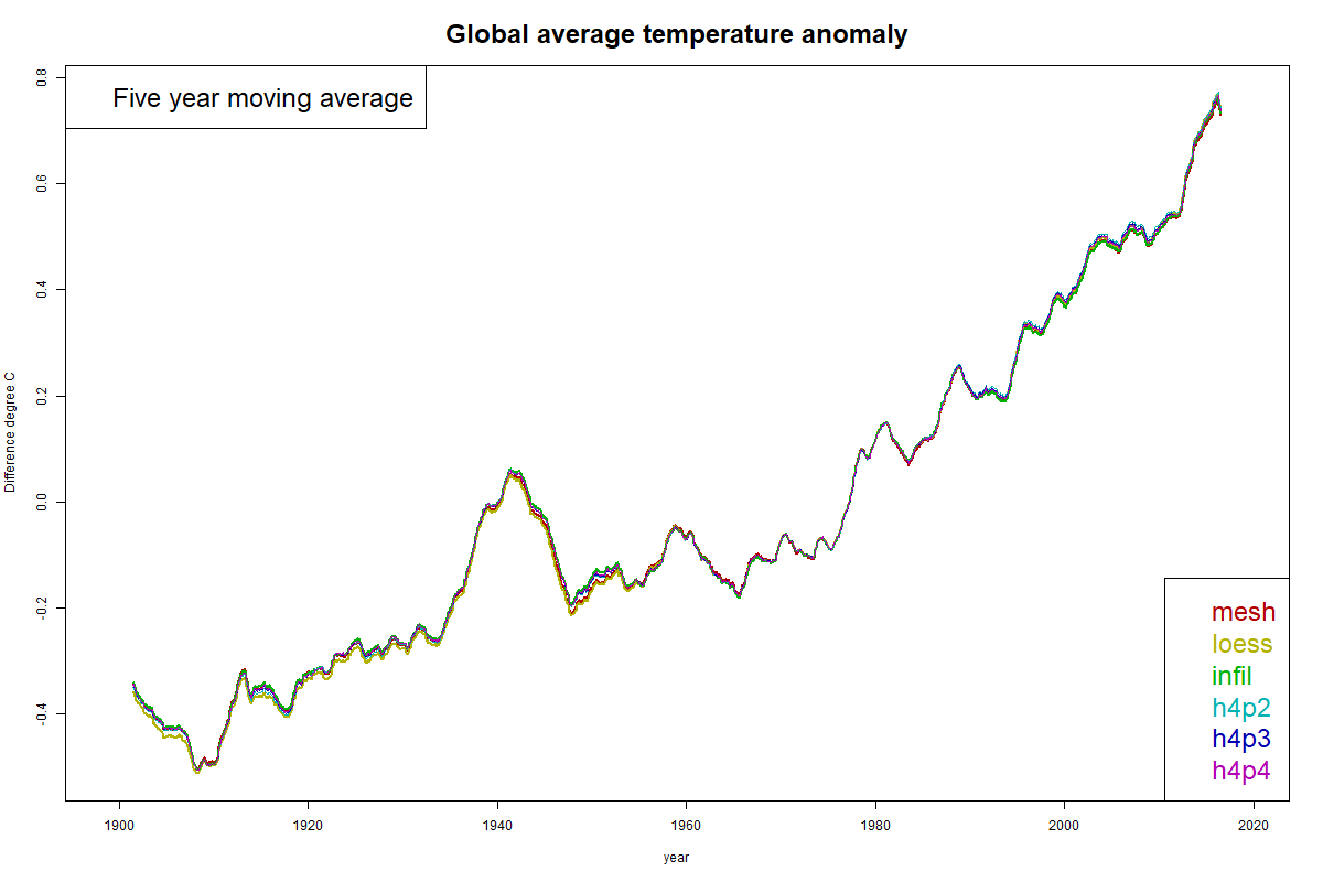
Difference plots are more informative. These are made by subtracting one of the solutions from the others. I have made plots using each of MESH, LOESS and INFILL as reference. You can click the buttons below the plot to cycle through.
There is a region of notably good agreement between 1960 and 1990. This is artificial, because that is the anomaly base period, so all plots have mean zero there. Still, they are unusually aligned in slope.
Before 1960, LOESS deviates from the FEM curves, MESH less, and INFILL least. The agreement of INFILL probably comes from the common use of Laplace interpolation for the empty Antarctic region. In the post 1990 period, it is LOESS which best tracks with FEM.
However, I should note that no discrepancies exceed about 0.02°C.
Mathematics of FEM/LOESS
It's actually a true hybrid of the finite element method (FEM) and LOESS (locally estimated scatterplot smoothing). In LOESS a model is fitted locally by regression, usually to get a central value. In FEM/LOESS, the following least squares parameter fit is made:The standard FEM approximate function is f(z)=ΣaᵢBᵢ(z) where z is location on the sphere, B are the basis functions described in the previous post, and aᵢ are the set of coefficients to be found by fitting to a set of observations that I will call y(z). The LS target is
SS=∫(f(z)-y(z))^2 dz
This has to be estimated knowing y at a discrete points (stations). In FEM style, the integral is split into integrals over elements, and then within elements the integrand is estimated as mean (f(zₖ)-y(zₖ))^2 over points k. One might question whether the sum within elements should be weighted, but the idea is that the fitted f() takes out the systematic variation, so the residuals should be homogeneous, and a uniform mean is correct.
So differentiating wrt a to minimise:
∫(f(z)-y(z))Bᵢ(z) dz = 0
Discretising:
Σₘ Eₘ (ΣₖBᵢ(zₖ)Bₙ(zₖ)aₙ)/(Σₖ1) = Σₘ Eₘ (ΣₖBᵢ(zₖ)yₖ)/(Σₖ1)
The first summation is over elements, and E are their areas. In FEM style, the summations that follow are specific to each element, and for each E include just the points zₖ within that element, and so the basis functions in the sum are those that have a node within or on the boundary if that element. The denominators Σₖ1 are just the count of points within each element. It looks complicated but putting it together is just the standard FEM step of assembling a mass matrix.
In symbols,this is the regression equation
H a = B* w B a = B* w y
where B is the matrix of basis functions evaluated at zₖ, B* transpose, diagonal matrix w the weights Σₘ/(Σₖ1) (area/count), y the vector of readings, and a the vector of unknown coefficients.
To integrate a specific y, this has to be solved for a:
a=H-1B* w y
and then ΣaᵢBᵢ(z) integrated on the globe
Int = ΣaᵢIᵢ where Iᵢ is the integral of function Bᵢ,
H is generally positive definite and sparse, so the inversion is done with conjugate gradients, using the diagonal as preconditioner.
For TempLS I need not an integral but weights. So I have to calculate
wt = I H-1B* w
It sounds hard, but it is a well trodden FEM task, and is computationally quite fast. In all this a small multiple of a Laplacian matrix is added to H to ensure corresponding infilling of empty or inadequately constrained cells.
Comparisons
I ran TempLS using the FEM/LOESS weighting with 9 modes, h2p2, h2p3, h2p4,...h43,h4p4. I calculated the RMS of differences between monthly averages, pairwise, for the years 1900-2019, and similar differences between and within the advanced methods MESH, LOESS and INFILL (see here for discussion, and explanation of the h..p.. notation). Here is a table of results, of RMS difference in °C, multiplied by 1000:| MESH | LOESS | INFILL | h2p2 | h3p2 | h4p2 | h5p2 | h2p3 | h3p3 | h4p3 | h5p3 | h2p4 | h3p4 | h4p4 | h5p4 | h2p5 | h3p5 | h4p5 | h5p5 | |
| MESH | 0 | 18 | 19 | 26 | 20 | 19 | 19 | 21 | 18 | 17 | 19 | 18 | 17 | 17 | 19 | 19 | 19 | 19 | 22 |
| LOESS | 18 | 0 | 25 | 24 | 22 | 19 | 22 | 20 | 22 | 20 | 23 | 19 | 22 | 21 | 24 | 22 | 23 | 24 | 27 |
| INFILL | 19 | 25 | 0 | 27 | 19 | 17 | 14 | 21 | 14 | 13 | 11 | 17 | 11 | 11 | 10 | 14 | 11 | 10 | 12 |
| h2p2 | 26 | 24 | 27 | 0 | 24 | 25 | 26 | 21 | 24 | 24 | 26 | 22 | 25 | 25 | 26 | 26 | 26 | 27 | 28 |
| h3p2 | 20 | 22 | 19 | 24 | 0 | 17 | 16 | 16 | 11 | 16 | 17 | 16 | 12 | 17 | 18 | 16 | 17 | 17 | 21 |
| h4p2 | 19 | 19 | 17 | 25 | 17 | 0 | 14 | 15 | 12 | 8 | 16 | 12 | 13 | 10 | 14 | 14 | 16 | 17 | 20 |
| h5p2 | 19 | 22 | 14 | 26 | 16 | 14 | 0 | 17 | 11 | 11 | 6 | 13 | 10 | 10 | 12 | 0 | 6 | 8 | 12 |
| h2p3 | 21 | 20 | 21 | 21 | 16 | 15 | 17 | 0 | 16 | 16 | 19 | 10 | 17 | 17 | 19 | 17 | 19 | 20 | 23 |
| h3p3 | 18 | 22 | 14 | 24 | 11 | 12 | 11 | 16 | 0 | 10 | 11 | 12 | 6 | 10 | 12 | 11 | 11 | 13 | 16 |
| h4p3 | 17 | 20 | 13 | 24 | 16 | 8 | 11 | 16 | 10 | 0 | 11 | 11 | 9 | 4 | 9 | 11 | 11 | 12 | 16 |
| h5p3 | 19 | 23 | 11 | 26 | 17 | 16 | 6 | 19 | 11 | 11 | 0 | 15 | 9 | 9 | 10 | 6 | 0 | 4 | 8 |
| h2p4 | 18 | 19 | 17 | 22 | 16 | 12 | 13 | 10 | 12 | 11 | 15 | 0 | 13 | 12 | 15 | 13 | 15 | 16 | 20 |
| h3p4 | 17 | 22 | 11 | 25 | 12 | 13 | 10 | 17 | 6 | 9 | 9 | 13 | 0 | 8 | 10 | 10 | 9 | 10 | 14 |
| h4p4 | 17 | 21 | 11 | 25 | 17 | 10 | 10 | 17 | 10 | 4 | 9 | 12 | 8 | 0 | 6 | 10 | 9 | 10 | 14 |
| h5p4 | 19 | 24 | 10 | 26 | 18 | 14 | 12 | 19 | 12 | 9 | 10 | 15 | 10 | 6 | 0 | 12 | 10 | 9 | 12 |
| h2p5 | 19 | 22 | 14 | 26 | 16 | 14 | 0 | 17 | 11 | 11 | 6 | 13 | 10 | 10 | 12 | 0 | 6 | 8 | 12 |
| h3p5 | 19 | 23 | 11 | 26 | 17 | 16 | 6 | 19 | 11 | 11 | 0 | 15 | 9 | 9 | 10 | 6 | 0 | 4 | 8 |
| h4p5 | 19 | 24 | 10 | 27 | 17 | 17 | 8 | 20 | 13 | 12 | 4 | 16 | 10 | 10 | 9 | 8 | 4 | 0 | 6 |
| h5p5 | 22 | 27 | 12 | 28 | 21 | 20 | 12 | 23 | 16 | 16 | 8 | 20 | 14 | 14 | 12 | 12 | 8 | 6 | 0 |
The best agreement between the older methods is between MESH and LOESS at 18. Agreement between the higher order FEM results is much better. Agreement of FEM with MESH is a little better, with LOESS a little worse. The agreement with INFILL is better again, but needs to be discounted somewhat. The reason is that in earlier years there is a large S Pole region without data. Both INFILL and FEM deal with this with Laplace interpolation, so I think that spuriously enhances the agreement.
As will be seen later, there is a change in the matchings at about 1960, when Antarctic data becomes available. So I did a similar table just for the years since 1960:
| MESH | LOESS | INFILL | h2p2 | h3p2 | h4p2 | h5p2 | h2p3 | h3p3 | h4p3 | h5p3 | h2p4 | h3p4 | h4p4 | h5p4 | h2p5 | h3p5 | h4p5 | h5p5 | |
| MESH | 0 | 11 | 11 | 23 | 17 | 16 | 14 | 18 | 13 | 12 | 12 | 15 | 12 | 11 | 10 | 14 | 12 | 12 | 16 |
| LOESS | 11 | 0 | 10 | 19 | 14 | 12 | 10 | 14 | 10 | 9 | 9 | 10 | 9 | 8 | 9 | 10 | 9 | 10 | 14 |
| INFILL | 11 | 10 | 0 | 21 | 16 | 16 | 13 | 17 | 13 | 12 | 11 | 15 | 11 | 10 | 9 | 13 | 11 | 10 | 13 |
| h2p2 | 23 | 19 | 21 | 0 | 20 | 20 | 20 | 18 | 20 | 20 | 20 | 18 | 20 | 20 | 21 | 20 | 20 | 20 | 22 |
| h3p2 | 17 | 14 | 16 | 20 | 0 | 15 | 15 | 13 | 10 | 14 | 15 | 13 | 11 | 14 | 16 | 15 | 15 | 15 | 19 |
| h4p2 | 16 | 12 | 16 | 20 | 15 | 0 | 12 | 12 | 10 | 7 | 14 | 9 | 10 | 9 | 13 | 12 | 14 | 16 | 20 |
| h5p2 | 14 | 10 | 13 | 20 | 15 | 12 | 0 | 15 | 11 | 9 | 6 | 11 | 10 | 10 | 11 | 0 | 6 | 8 | 13 |
| h2p3 | 18 | 14 | 17 | 18 | 13 | 12 | 15 | 0 | 12 | 13 | 16 | 10 | 13 | 14 | 16 | 15 | 16 | 17 | 20 |
| h3p3 | 13 | 10 | 13 | 20 | 10 | 10 | 11 | 12 | 0 | 9 | 12 | 8 | 6 | 9 | 11 | 11 | 12 | 13 | 17 |
| h4p3 | 12 | 9 | 12 | 20 | 14 | 7 | 9 | 13 | 9 | 0 | 10 | 9 | 7 | 4 | 8 | 9 | 10 | 11 | 16 |
| h5p3 | 12 | 9 | 11 | 20 | 15 | 14 | 6 | 16 | 12 | 10 | 0 | 13 | 9 | 9 | 9 | 6 | 0 | 4 | 9 |
| h2p4 | 15 | 10 | 15 | 18 | 13 | 9 | 11 | 10 | 8 | 9 | 13 | 0 | 9 | 9 | 12 | 11 | 13 | 14 | 18 |
| h3p4 | 12 | 9 | 11 | 20 | 11 | 10 | 10 | 13 | 6 | 7 | 9 | 9 | 0 | 7 | 9 | 10 | 9 | 11 | 15 |
| h4p4 | 11 | 8 | 10 | 20 | 14 | 9 | 10 | 14 | 9 | 4 | 9 | 9 | 7 | 0 | 6 | 10 | 9 | 10 | 15 |
| h5p4 | 10 | 9 | 9 | 21 | 16 | 13 | 11 | 16 | 11 | 8 | 9 | 12 | 9 | 6 | 0 | 11 | 9 | 9 | 13 |
| h2p5 | 14 | 10 | 13 | 20 | 15 | 12 | 0 | 15 | 11 | 9 | 6 | 11 | 10 | 10 | 11 | 0 | 6 | 8 | 13 |
| h3p5 | 12 | 9 | 11 | 20 | 15 | 14 | 6 | 16 | 12 | 10 | 0 | 13 | 9 | 9 | 9 | 6 | 0 | 4 | 9 |
| h4p5 | 12 | 10 | 10 | 20 | 15 | 16 | 8 | 17 | 13 | 11 | 4 | 14 | 11 | 10 | 9 | 8 | 4 | 0 | 7 |
| h5p5 | 16 | 14 | 13 | 22 | 19 | 20 | 13 | 20 | 17 | 16 | 9 | 18 | 15 | 15 | 13 | 13 | 9 | 7 | 0 |
Clearly the agreement is much better. The best of the older methods is between LOESS and INFILL at 10. But agreement between high order FEM methods is better. Now it is LOESS that agrees well with FEM - better than the others. Of course in assessing agreement, we don't know which is right. It is possible that FEM is the best, but not sure.
Here are some time series graphs. I'll show a time series graph first, but the solutions are too close to distinguish much.
Difference plots are more informative. These are made by subtracting one of the solutions from the others. I have made plots using each of MESH, LOESS and INFILL as reference. You can click the buttons below the plot to cycle through.
There is a region of notably good agreement between 1960 and 1990. This is artificial, because that is the anomaly base period, so all plots have mean zero there. Still, they are unusually aligned in slope.
Before 1960, LOESS deviates from the FEM curves, MESH less, and INFILL least. The agreement of INFILL probably comes from the common use of Laplace interpolation for the empty Antarctic region. In the post 1990 period, it is LOESS which best tracks with FEM.
However, I should note that no discrepancies exceed about 0.02°C.
Next steps
After further experience, I will probably make FEM/LOESS my frontline method.Wednesday, October 16, 2019
GISS September global unchanged from August.
The GISS V4 land/ocean temperature anomaly stayed at 0.90°C in September, same as August. It compared with a 0.043deg;C fall in TempLS V4 mesh
The overall pattern was similar to that in TempLS. Warm in Africa, N of China, Eastern US, NE Pacific, Alaska/Arctic. Cool over Urals, in West Coast USA and Atlantic Canada. Mostly cool in Antarctica.
As usual here, I will compare the GISS and earlier TempLS plots below the jump.
The overall pattern was similar to that in TempLS. Warm in Africa, N of China, Eastern US, NE Pacific, Alaska/Arctic. Cool over Urals, in West Coast USA and Atlantic Canada. Mostly cool in Antarctica.
As usual here, I will compare the GISS and earlier TempLS plots below the jump.
Monday, October 14, 2019
New FEM/LOESS method of integrating temperature anomalies on the globe
Update Correction to sensitivity to rotation below
Yet another post on this topic, which I have written a lot about. It is the the basis of calculation of global temperature anomaly, which I do every month with TempLS. I have developed three methods that I consider advanced, and I post averages using each here (click TempLS tab). They agree fairly well, and I think they are all satisfactory (and better than the alternatives in common use). The point of developing three was partly that they are based on different principles, and yet give concordant results. Since we don't have an exact solution to check against, that is the next best thing.
So why another one? Despite their good results, the methods have strong points and some imperfections. I would like a method that combines the virtues of the three, and sheds some faults. A bonus would be that it runs faster. I think I have that here. I'll call it the FEM method, since it makes more elaborate use of finite element ideas. I'll first briefly describe the existing methods and their pros and cons.
Mesh method
This has been my mainstay for about eight years. For each month an irregular triangular mesh (convex hull) is drawn connecting the stations that reported. The function formed by linear interpolation within each triangle is integrated. The good thing about the method is that it adapts well to varying coverage, giving the (near) best even where sparse. One bad thing is the different mesh for each month, which takes time to calculate (if needed) and is bulky to put online for graphics. The time isn't much; about an hour in full for GHCN V4, but I usually store geometry data for past months, which can reduce process time to a minute or so. But GHCN V4 is apt to introduce new stations, which messes up my storage.A significant point is that the mesh method isn't stochastic, even though the data is best thought of as having a random component. By that I mean that it doesn't explicitly try to integrate an estimated average, but relies o exact integration to average out. It does, generally, very well. But a stochastic method gives more control, and is alos more efficient.
Grid method with infill
Like most people, I started with a lat/lon grid, averaging station values within each cell, and then an area-weighted average of cells. This has a big problem with empty cells (no data) and so I developed infill schemes to estimate those from local dat. Here is an early description of a rather ad hoc method. Later I got more systematic about it, eventually solving a Laplace equation for empty cell regions, using data cells as boundary conditions.The method is good for averaging, and reasonably fast. It is stochastic, in the cell averaging step. But I see it now in finite element terms, and it uses a zero order representation within the cell (constant), with discontinuity at the boundary. In FEM, such an element would be scorned. We can do better. It is also not good for graphics.,
LOESS method
My third, and most recent method, is described here. It starts with a regular icosahedral grid of near uniform density. LOESS (local weighted linear regression) is used to assign values to the nodes of that grid, and an interpolation function (linear mesh) is created on that grid which is either integrated or used for graphics. It is accurate and gives the best graphics.Being LOESS, it is explicitly stochastic. I use an exponential weighting function derived from Hansen's spatial correlation decay, but a more relevant cut-off is that for each node I choose the nearest 20 points to average. There are some practical reasons for this. An odd side effect is that about a third of stations do not contribute; they are in dense regions where they don't make the nearest 20 of any node. This is in a situation of surfeit of information, but it seems a pity to not use their data in some way.
The new FEM method.
I take again a regular triangle grid based on subdividing the icosahedron (projected onto the sphere). Then I form polynomial basis functions of some order (called P1, P2 etc in the trade). These have generally a node for each function, of which there may be several per triangle element - the node arrangement within triangles are shown in a diagram below. The functions are "tent-like", and go to zero on the boundaries, unless the node is common to several elements, in which case it is zero on the boundary of that set of elements and beyond. They have the property of being one at the centre and zero at all other nodes, so if you have a function with values at the node, multiplying those by the basis functions and adding forms a polynomial interpolation of appropriate order, which can be integrated or graphed. Naturally, there is a WebGL visualisation of these shape functions; see at the end.The next step is somewhat nonstandard FEM. I use the basis functions as in LOESS. That is, I require that the interpolating will be a best least squares fit to the data at its scattered stations. This is again local regression. But the advantage over the above LOESS is that the basis functions have compact support. That is, you only have to regress, for each node, data within the elements of which the node is part.
Once that is done, the regression expressions are aggregated as in finite element assembly, to produce the equivalent of a mass matrix which has to be inverted. The matrix can be large but it is sparse (most element zero). It is also positive definite and well conditioned, so I can use a preconditioned conjugate gradient method to solve. This converges quickly.
Advantages of the method
- Speed - binning of nodes is fast compared to finding pairwise distances as in LOESS, and furthermore it can be done just once for the whole inventory. Solution is very fast.
- Graphics - the method explicitly creates an interpolation method.
- Convergence - you can look at varying subdivision (h) and polynomial order of basis (p). There is a powerful method in FEM of hp convergence, which says that if you improve h and p jointly on some way, you get much faster convergence than improving one with the other fixed.
Failure modes
The method eventually fails when elements don't have enough data to constrain the parameters (node values) that are being sought. This can happen either because the subdivision is too fine (near empty cells) or the order of fitting is too high for the available data. This is a similar problem to the empty cells in simple gridding, and there is a simple solution, which limits bad consequences, so missing data in one area won't mess up the whole integral. The specific fault is that the global matrix to be inverted becomes ill-conditioned (near-singular) so there are spurious modes from its null space that can grow. The answer is to add a matrix corresponding to a Laplacian, with a small multiplier. The effect of this is to say that where a region is unconstrained, a smoothness constraint is added. A light penalty is put on rapid change at the boundaries. This has little effect on the non-null space of the mass matrix, but means that the smoothness requirement becomes dominant where other constraints fail. This is analogous to the Laplace infilling I now do with the grid method.Comparisons and some results
I have posted comparisons of the various methods used with global time series above and others, most recently here. Soon I will do the same for these methods, but for now I just want to show how the hp-system converges. Here is the listing of global averages of anomalies calculated by the mesh method for February to July, 2019. I'll use the FEM hp notation, where h1 is the original icosahedron, and higher orders hn have each triangle divided into n², so h4 has 320 triangles. p represents polynomial order, so p1 is linear, p2 quadratic.
|
|
| ||||||||||||||||||||||||||||||||||||||||||||||||||||||||||||||||||||||||||||||||||||||||||
|
|
| ||||||||||||||||||||||||||||||||||||||||||||||||||||||||||||||||||||||||||||||||||||||||||
Note that h1p1 is the main outlier. But the best convergence is toward bottom right.
Sensitivity analysis
Update Correction - I made a programming error with the numbers that appeared here earlier. The new numbers are larger, making significant uncertainty in the third decimal place at best, and more for h1.
I did a test of how sensitive the result was to placement of the icosahedral mesh. For the three months May-July, I took the original placement of the icosahedron, with vertex at the N pole, and rotated about each axis successively by random angles. I did this 50 times, and computed the standard deviations of the results. Here they are, multiplied by a million:
|
|
| |||||||||||||||||||||||||||||||||||||||||||||||||||||||||||||||||||||||||||||||||||||||||||||
The error affects the third decimal place
Convergent plots
Here is a collection of plots for the various hp pairs in the table, for the month of July. The resolution goes from poor to quite good. But you don't need very high resolution for a global integral. Click the arrow buttons below to cycle through.Visualisation of shape functions
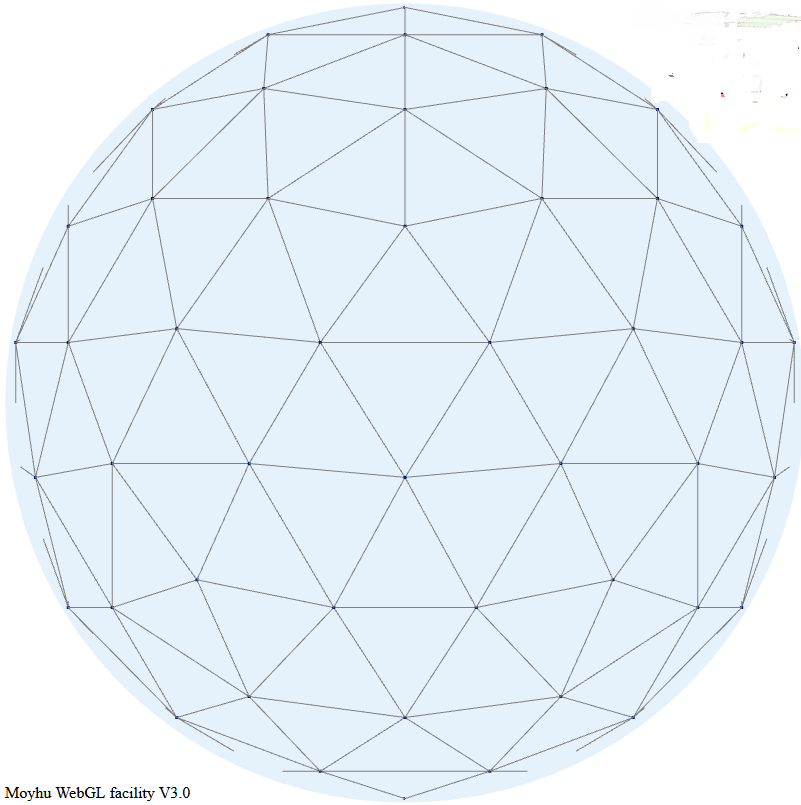
A shape functions is, within a triangle, the unique polynomial of appropriate order which take value 1 at their node, and zero at all other nodes. The arrangement of these nodes is shown below: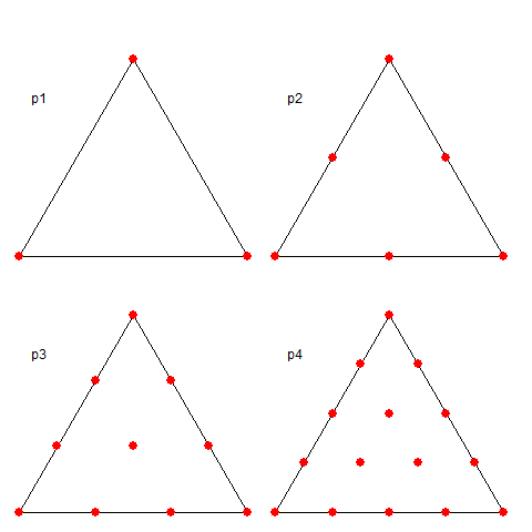
Here is a visualisation of some shape functions. Each is nonzero over just a few triangles in the icosahedron mesh. Vertex functions have a hexagon base, being the six triangles to which the vertex is common. Functions centered on a side have just the two adjacent triangles as base. Higher order elements also have internal functions over just the one triangle, which I haven't shown. The functions are zero in the mesh beyond their base, as shown with grey. The colors represent height above zero, so violet etc is usually negative.
It is the usual Moyhu WebGL plot, so you can drag with the mouse to move it about. The radio buttons allow you to vary the shape function in view, using the hnpn notation from above.
Next step
For use in TempLS, the integration method needs to be converted to return weights for integrating the station values. This has been done and in the next post I will compare time series plots for the three existing advanced methods and the new FEM method with the range of hp values.Tuesday, October 8, 2019
September global surface TempLS down 0.043°C from August.
The TempLS mesh anomaly (1961-90 base) was 0.758deg;C in September vs 0.801°C in August. This contrasts with the 0.03°C rise in the NCEP/NCAR reanalysis base index. This makes it the second warmest September in the record, just behind 2016.
SST was down somewhat, mainly due to far Southern Ocean. There was also a cool area north of Australia, and in Russia around the Urals. Most of US was warm, except the Pacific coast; E Canada was cool. There were warm areas N of China, in S America E of Bolivia, and Alaska/E Siberia. Africa was warm.
There was a sharp rise of about 0.2°C in satellite indices, which Roy Spencer attributes to stratospheric warming over Antarctica. TempLS found that Antarctica was net cool at surface, although it shows as rather warm on the lat/lon map. As always, the 3D globe map gives better detail.
Here is the temperature map, using the LOESS-based map of anomalies.
Thursday, October 3, 2019
September NCEP/NCAR global surface anomaly up 0.03°C from August
The Moyhu NCEP/NCAR index rose from 0.389°C in August to 0.419°C in September, on a 1994-2013 anomaly base. It continued the pattern of the last three months of small rises with only small excursions during the month. In fact there hasn't really been a cold spell globally since February, which is unusual. It is the warmest September since 2016 in this record.
N America was warm E of Rockies, colder W, but warm toward Alaska, extending across N of Siberia.. A large cool atch ar in N Australia and further N. Mostly cool in and around Antarctica. A warm patch N of China.
N America was warm E of Rockies, colder W, but warm toward Alaska, extending across N of Siberia.. A large cool atch ar in N Australia and further N. Mostly cool in and around Antarctica. A warm patch N of China.
Tuesday, September 17, 2019
GISS August global down 0.04°C from July.
The GISS V4 land/ocean temperature anomaly fell 0.04°C in August. The anomaly average was 0.90°C, down from July 0.94°C. It compared with a 0.029°C fall in TempLS V4 mesh
The overall pattern was similar to that in TempLS. Warm in Africa, N central Siberia, NE Canada, NE Pacific. Cool in a band from US Great Lakes to NW Canada and in NW Russia. Mostly warm in Antarctica.
As usual here, I will compare the GISS and earlier TempLS plots below the jump.
The overall pattern was similar to that in TempLS. Warm in Africa, N central Siberia, NE Canada, NE Pacific. Cool in a band from US Great Lakes to NW Canada and in NW Russia. Mostly warm in Antarctica.
As usual here, I will compare the GISS and earlier TempLS plots below the jump.
Wednesday, September 11, 2019
How errors really propagate in differential equations (and GCMs).
There has been more activity on Pat Frank's paper since my last post. A long thread at WUWT, with many comments from me. And two good posts and threads at ATTP, here and here. In the latter he coded up Pat's simple form (paper here). Roy Spencer says he'll post a similar effort in the morning. So I thought writing something on how error really is propagated in differential equations would be timely. It's an absolutely core part of PDE algorithms, since it determines stability. And it isn't simple, but expresses important physics. Here is a TOC:
A partial differential equation system, as in a GCM, has derivatives in several variables, usually space and time. In computational fluid dynamics (CFD) of which GCMs are part, the space is gridded into cells or otherwise discretised, with variables associated with each cell, or maybe nodes. The system is stepped forward in time. At each stage there are a whole lot of spatial relations between the discretised variables, so it works like a time de with a huge number of cell variables and relations. That is for explicit solution, which is often used by large complex systems like GCMs. Implicit solutions stop to enforce the space relations before proceeding.
Solutions of a first order equation are determined by their initial conditions, at least in the short term. A solution beginning from a specific state is called a trajectory. In a linear system, and at some stage there is linearisation, the trajectories form a linear space with a basis corresponding to the initial variables.
It is said, often in disparagement of GCMs, that they are not effectively determined by initial conditions. A small change in initial state could give a quite different solution. Put in terms of what is said above, they can't stay on a single trajectory.
That is true, and true in CFD, but it is a feature, not a bug, because we can hardly ever determine the initial conditions anyway, even in a wind tunnel. And even if we could, there is no chance in an aircraft during flight, or a car in motion. So if we want to learn anything useful about fluids, either with CFD or a wind tunnel, it will have to be something that doesn't require knowing initial conditions.
Of course, there is a lot that we do want to know. With an aircraft wing, for example, there is lift and drag. These don't depend on initial conditions, and are applicable throughout the flight. With GCMs it is climate that we seek. The reason we can get this knowledge is that, although we can't stick to any one of those trajectories, they are all subject to the same requirements of mass, momentum and energy conservation, and so in bulk all behave in much the same way (so it doesn't matter where you started). Practical information consists of what is common to a whole bunch of trajectories.
Turbulence messes up the neat idea of trajectories, but not too much, because of Reynolds Averaging. I won't go into this except to say that it is possible to still solve for a mean flow, which still satisfies mass momentum etc. It will be a useful lead in to the business of error propagation, because it is effectively a continuing source of error.
As said, turbulence can be seen as a continuing source of error. But it doesn't grow without limit. A common model of turbulence is called k-ε. k stands for turbulent kinetic energy, ε for rate of dissipation. There are k source regions (boundaries), and diffusion equations for both quantities. The point is that the result is a balance. Turbulence overall dissipates as fast as it is generated. The reason is basically conservation of angular momentum in the eddies of turbulence. It can be positive or negative, and diffuses (viscosity), leading to cancellation. Turbulence stays within bounds.
But, I hear, how is that different from extra GHG? The reason is that GHGs don't create a single burst of flux; they create an ongoing flux, shifting the solution long term. Of course, it is possible that cloud cover might vary long term too. That would indeed be a forcing, as is acknowledged. But fluctuations, as expressed in the 4 W/m2 uncertainty of Pat Frank (from Lauer) will dissipate through conservation.
It is of the common kind, in effect a first order de
d( ΔT)/dt = a F
where F is a combination of forcings. It is said to emulate well the GCM solutions; in fact Pat Frank picks up a fallacy common at WUWT that if a GCM solution (for just one of its many variables) turns out to be able to be simply described, then the GCM must be trivial. This is of course nonsense - the task of the GCM is to reproduce reality in some way. If some aspect of reality has a pattern that makes it predictable, that doesn't diminish the GCM.
The point is, though, that while the simple equation may, properly tuned, follow the GCM, it does not have alternative trajectories, and more importantly does not obey physical conservation laws. So it can indeed go off on a random walk. There is no correspondence between the error propagation of Eq 1 (random walk) and the GCMs (shift between solution trajectories of solutions of the Navier-Stokes equations, conserving mass momentum and energy).
"Scientific models are held to the standard of mortal tests and successful predictions outside any calibration bound. The represented systems so derived and tested must evolve congruently with the real-world system if successful predictions are to be achieved."
That just isn't true. They are models of the Earth, but they don't evolve congruently with it (or with each other). They respond like the Earth does, including in both cases natural variation (weather) which won't match. As the IPCC says:
"In climate research and modelling, we should recognise that we are dealing with a coupled non-linear chaotic system, and therefore that the long-term prediction of future climate states is not possible. The most we can expect to achieve is the prediction of the probability distribution of the system’s future possible states by the generation of ensembles of model solutions. This reduces climate change to the discernment of significant differences in the statistics of such ensembles"
If the weather doesn't match, the fluctuations of cloud cover will make no significant difference on the climate scale. A drift on that time scale might, and would then be counted as a forcing, or feedback, depending on cause.
- Differential equations
- Fluids and Turbulence
- Error propagation
- GCM errors and conservation
- Simple equation analogies
- On Earth models
- Conclusion
Differential equations
An ordinary differential equation (de) system is a number of equations relating many variables and their derivatives. Generally the number of variables and equations is equal. There could be derivatives of higher order, but I'll restrict to one, so it is a first order system. Higher order systems can always be reduced to first order with extra variables and corresponding equations.A partial differential equation system, as in a GCM, has derivatives in several variables, usually space and time. In computational fluid dynamics (CFD) of which GCMs are part, the space is gridded into cells or otherwise discretised, with variables associated with each cell, or maybe nodes. The system is stepped forward in time. At each stage there are a whole lot of spatial relations between the discretised variables, so it works like a time de with a huge number of cell variables and relations. That is for explicit solution, which is often used by large complex systems like GCMs. Implicit solutions stop to enforce the space relations before proceeding.
Solutions of a first order equation are determined by their initial conditions, at least in the short term. A solution beginning from a specific state is called a trajectory. In a linear system, and at some stage there is linearisation, the trajectories form a linear space with a basis corresponding to the initial variables.
Fluids and Turbulence
As in CFD, GCMs solve the Navier-Stokes equations. I won't spell those out (I have an old post here), except to say that they simply express the conservation of momentum and mass, with an addition for energy. That is, a version of F=m*a, and an equation expressing how the fluid relates density and velocity divergence (and so pressure with a constitutive equation), and an associated heat budget equation.It is said, often in disparagement of GCMs, that they are not effectively determined by initial conditions. A small change in initial state could give a quite different solution. Put in terms of what is said above, they can't stay on a single trajectory.
That is true, and true in CFD, but it is a feature, not a bug, because we can hardly ever determine the initial conditions anyway, even in a wind tunnel. And even if we could, there is no chance in an aircraft during flight, or a car in motion. So if we want to learn anything useful about fluids, either with CFD or a wind tunnel, it will have to be something that doesn't require knowing initial conditions.
Of course, there is a lot that we do want to know. With an aircraft wing, for example, there is lift and drag. These don't depend on initial conditions, and are applicable throughout the flight. With GCMs it is climate that we seek. The reason we can get this knowledge is that, although we can't stick to any one of those trajectories, they are all subject to the same requirements of mass, momentum and energy conservation, and so in bulk all behave in much the same way (so it doesn't matter where you started). Practical information consists of what is common to a whole bunch of trajectories.
Turbulence messes up the neat idea of trajectories, but not too much, because of Reynolds Averaging. I won't go into this except to say that it is possible to still solve for a mean flow, which still satisfies mass momentum etc. It will be a useful lead in to the business of error propagation, because it is effectively a continuing source of error.
Error propagation and turbulence
I said that in a first order system, there is a correspondence between states and trajectories. That is, error means that the state isn't what you thought, and so you have shifted to a different trajectory. But, as said, we can't follow trajectories for long anyway, so error doesn't really change that situation. The propagation of error depends on how the altered trajectories differ. And again, because of the requirements of conservation, they can't differ by all that much.As said, turbulence can be seen as a continuing source of error. But it doesn't grow without limit. A common model of turbulence is called k-ε. k stands for turbulent kinetic energy, ε for rate of dissipation. There are k source regions (boundaries), and diffusion equations for both quantities. The point is that the result is a balance. Turbulence overall dissipates as fast as it is generated. The reason is basically conservation of angular momentum in the eddies of turbulence. It can be positive or negative, and diffuses (viscosity), leading to cancellation. Turbulence stays within bounds.
GCM errors and conservation
In a GCM something similar happens with other perurbations. Suppose for a period, cloud cover varies, creating an effective flux. That is what Pat Frank's paper is about. But that flux then comes into the general equilibrating processes in the atmosphere. Some will go into extra TOA radiation, some into the sea. It does not accumulate in random walk fashion.But, I hear, how is that different from extra GHG? The reason is that GHGs don't create a single burst of flux; they create an ongoing flux, shifting the solution long term. Of course, it is possible that cloud cover might vary long term too. That would indeed be a forcing, as is acknowledged. But fluctuations, as expressed in the 4 W/m2 uncertainty of Pat Frank (from Lauer) will dissipate through conservation.
Simple Equation Analogies
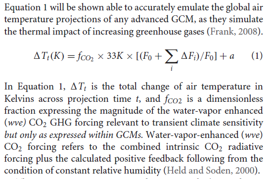
Pat Frank, of course, did not do anything with GCMs. Instead he created a simple model, given by his equation 1:
It is of the common kind, in effect a first order de
d( ΔT)/dt = a F
where F is a combination of forcings. It is said to emulate well the GCM solutions; in fact Pat Frank picks up a fallacy common at WUWT that if a GCM solution (for just one of its many variables) turns out to be able to be simply described, then the GCM must be trivial. This is of course nonsense - the task of the GCM is to reproduce reality in some way. If some aspect of reality has a pattern that makes it predictable, that doesn't diminish the GCM.
The point is, though, that while the simple equation may, properly tuned, follow the GCM, it does not have alternative trajectories, and more importantly does not obey physical conservation laws. So it can indeed go off on a random walk. There is no correspondence between the error propagation of Eq 1 (random walk) and the GCMs (shift between solution trajectories of solutions of the Navier-Stokes equations, conserving mass momentum and energy).
On Earth models
I'll repeat something here from the last post; Pat Frank has a common misconception about the function of GCM's. He says that"Scientific models are held to the standard of mortal tests and successful predictions outside any calibration bound. The represented systems so derived and tested must evolve congruently with the real-world system if successful predictions are to be achieved."
That just isn't true. They are models of the Earth, but they don't evolve congruently with it (or with each other). They respond like the Earth does, including in both cases natural variation (weather) which won't match. As the IPCC says:
"In climate research and modelling, we should recognise that we are dealing with a coupled non-linear chaotic system, and therefore that the long-term prediction of future climate states is not possible. The most we can expect to achieve is the prediction of the probability distribution of the system’s future possible states by the generation of ensembles of model solutions. This reduces climate change to the discernment of significant differences in the statistics of such ensembles"
If the weather doesn't match, the fluctuations of cloud cover will make no significant difference on the climate scale. A drift on that time scale might, and would then be counted as a forcing, or feedback, depending on cause.
Conclusion
Error propagation in differential equations follows the solution trajectories of the differential equations, and can't be predicted without it. With GCMs those trajectories are constrained by the requirements of conservation of mass, momentum and energy, enforced at each timestep. Any process which claims to emulate that must emulate the conservation requirements. Pat Frank's simple model does not.Sunday, September 8, 2019
Another round of Pat Frank's "propagation of uncertainties.
See update below for a clear and important error.
There has been another round of the bizarre theories of Pat Frank, saying that he has found huge uncertainties in GCM outputs that no-one else can see. His paper has found a publisher - WUWT article here. It is a pinned article; they think it is a big deal.
The paper is in Frontiers or Earth Science. This is an open publishing system, with (mostly) named reviewers and editors. The supportive editor was Jing-Jia Luo, who has been at BoM but is now at Nanjing. The named reviewers are Carl Wunsch and Davide Zanchettin.
I wrote a Moyhu article on this nearly two years ago, and commented extensively on WUWT threads, eg here. My objections still apply. The paper is nuts. Pat Frank is one of the hardy band at WUWT who insist that taking a means of observations cannot improve the original measurement uncertainty. But he takes it further, as seen in the neighborhood of his Eq 2. He has a cloud cover error estimated annually over 20 years. He takes the average, which you might think was just a average of error. But no, he insists that if you average annual data, then the result is not in units of that data, but in units/year. There is a wacky WUWT to-and-fro on that beginning here. A referee had objected to changing the units of annual time series averaged data by inserting the /year. The referee probably thought he was just pointing out an error that would be promptly corrected. But no, he coped a tirade about his ignorance. And it's true that it is not a typo, but essential to the arithmetic. Having given it units/year, that makes it a rate that he accumulates. I vainly pointed out that if he had gathered the data monthly instead of annually, the average would be assigned units/month, not /year, and then the calculated error bars would be sqrt(12) times as wide.
One thing that seems newish is the emphasis on emulation. This is also a WUWT strand of thinking. You can devise simple time models, perhaps based on forcings, which will give similar results to GCMs for one particular variable, global averaged surface temperature anomaly. So, the logic goes, that must be what GCM's are doing (never mind all the other variables they handle). And Pat Frank's article has much of this. From the abstract: "An extensive series of demonstrations show that GCM air temperature projections are just linear extrapolations of fractional greenhouse gas (GHG) forcing." The conclusion starts: "This analysis has shown that the air temperature projections of advanced climate models are just linear extrapolations of fractional GHG forcing." Just totally untrue, of course, as anyone who actually understands GCMs would know.
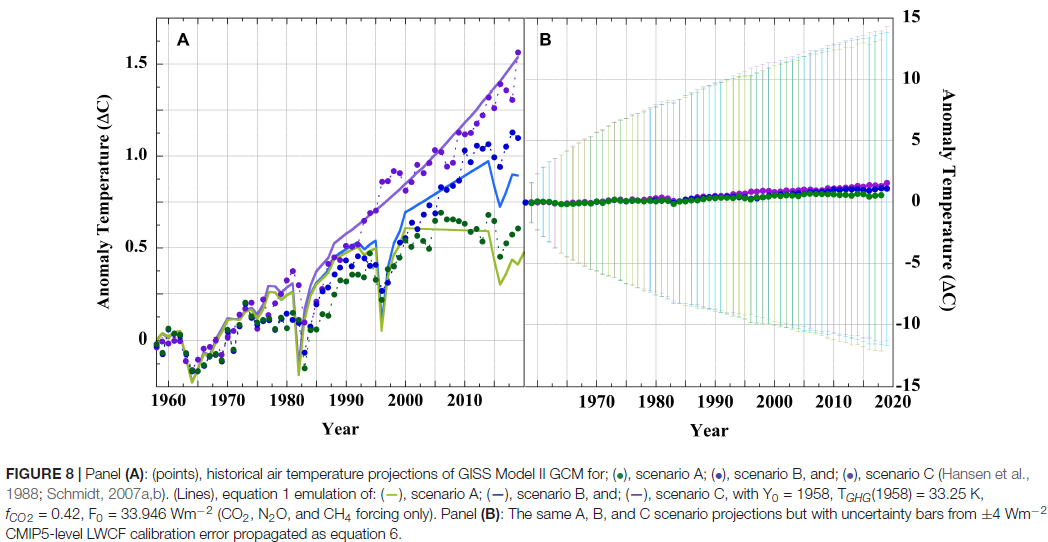
One funny thing - I pointed out here that PF's arithmetic would give a ±9°C error range in Hansen's prediction over 30 years. Now I argue that Hansen's prediction was good; some object that it was out by a small fraction of a degree. It would be an odd view that he was extraordinarily lucky to get such a good prediction with those uncertainties. But what do I see? This is now given, not as a reduction ad absurdum, but with a straight face as Fig 8:
To give a specific example of this nutty arithmetic, the paper deals with cloud cover uncertainty thus:
"On conversion of the above CMIP cloud RMS error (RMSE) as ±(cloud-cover unit) year-1 model-1 into a longwave cloud-forcing uncertainty statistic, the global LWCF calibration RMSE becomes ±Wm-2 year-1 model-1. Lauer and Hamilton reported the CMIP5 models to produce an annual average LWCF root-mean-squared error (RMSE) = ±4 Wm-2 year-1 model-1, relative to the observational cloud standard (81). This calibration error represents the average annual uncertainty within the simulated tropospheric thermal energy flux and is generally representative of CMIP5 models."
There is more detailed discussion of this starting here. In fact, Lauer and Hamilton said, correctly, that the RMSE was 4 Wm-2. The year-1 model-1 is nonsense added by PF, but it has an important effect. The year-1 translates directly into the amount of error claimed. If it had been month-1, the claim would have been sqrt(12) higher. So why choose year? PF's only answer - because L&H chose to bin their data annually. That determines GCM uncertainty!
Actually, the ±4 is another issue, explored here. Who writes an RMS as ±4? It's positive. But again it isn't just a typo. An editor in his correspondence, James Annan wrote it as 4, and was blasted as an ignorant sod for omitting the ±. I pointed out that no-one, nor L&H in his reference, used a ± for RMS. It just isn't the meaning of the term. I challenged him to find that usage anywhere, with no result. Unlike the nutty units, I think this one doesn't affect the arithmetic. It's just an indication of being in a different world.
One final thing I should mention is the misunderstanding of climate models contained in the preamble. For example "Scientific models are held to the standard of mortal tests and successful predictions outside any calibration bound. The represented systems so derived and tested must evolve congruently with the real-world system if successful predictions are to be achieved."
But GCMs are models of the earth. They aim to have the same physical properties but are not expected to evolve congruently, just as they don't evolve congruently with each other. This was set out in the often misquoted IPCC statement
"In climate research and modelling, we should recognise that we are dealing with a coupled non-linear chaotic system, and therefore that the long-term prediction of future climate states is not possible. The most we can expect to achieve is the prediction of the probability distribution of the system’s future possible states by the generation of ensembles of model solutions. This reduces climate change to the discernment of significant differences in the statistics of such ensembles. "
Update - I thought I might just highlight this clear error resulting from the nuttiness of the /year attached to averaging. It's from p 12 of the paper: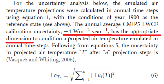
Firstly, of course, they are not the dimensions (Wm-2) given by the source, Lauer and Hamilton. But the dimensions don't work anyway. The sum of squares gives a year-2 dimension component. Then just taking the sqrt brings that back to year-1. But that is for the uncertainty of the whole period, so that can't be right. I assume Pat Frank puts his logic backward, saying that adding over 20 years multiplies the dimensions by year. But that still leaves the dimension (Wm-2)2 year-1, and on taking sqrt, the unit is (Wm-2)year-1/2. Still makes no sense; the error for a fixed 20 year period should be Wm-2.
There has been another round of the bizarre theories of Pat Frank, saying that he has found huge uncertainties in GCM outputs that no-one else can see. His paper has found a publisher - WUWT article here. It is a pinned article; they think it is a big deal.
The paper is in Frontiers or Earth Science. This is an open publishing system, with (mostly) named reviewers and editors. The supportive editor was Jing-Jia Luo, who has been at BoM but is now at Nanjing. The named reviewers are Carl Wunsch and Davide Zanchettin.
I wrote a Moyhu article on this nearly two years ago, and commented extensively on WUWT threads, eg here. My objections still apply. The paper is nuts. Pat Frank is one of the hardy band at WUWT who insist that taking a means of observations cannot improve the original measurement uncertainty. But he takes it further, as seen in the neighborhood of his Eq 2. He has a cloud cover error estimated annually over 20 years. He takes the average, which you might think was just a average of error. But no, he insists that if you average annual data, then the result is not in units of that data, but in units/year. There is a wacky WUWT to-and-fro on that beginning here. A referee had objected to changing the units of annual time series averaged data by inserting the /year. The referee probably thought he was just pointing out an error that would be promptly corrected. But no, he coped a tirade about his ignorance. And it's true that it is not a typo, but essential to the arithmetic. Having given it units/year, that makes it a rate that he accumulates. I vainly pointed out that if he had gathered the data monthly instead of annually, the average would be assigned units/month, not /year, and then the calculated error bars would be sqrt(12) times as wide.
One thing that seems newish is the emphasis on emulation. This is also a WUWT strand of thinking. You can devise simple time models, perhaps based on forcings, which will give similar results to GCMs for one particular variable, global averaged surface temperature anomaly. So, the logic goes, that must be what GCM's are doing (never mind all the other variables they handle). And Pat Frank's article has much of this. From the abstract: "An extensive series of demonstrations show that GCM air temperature projections are just linear extrapolations of fractional greenhouse gas (GHG) forcing." The conclusion starts: "This analysis has shown that the air temperature projections of advanced climate models are just linear extrapolations of fractional GHG forcing." Just totally untrue, of course, as anyone who actually understands GCMs would know.
One funny thing - I pointed out here that PF's arithmetic would give a ±9°C error range in Hansen's prediction over 30 years. Now I argue that Hansen's prediction was good; some object that it was out by a small fraction of a degree. It would be an odd view that he was extraordinarily lucky to get such a good prediction with those uncertainties. But what do I see? This is now given, not as a reduction ad absurdum, but with a straight face as Fig 8:
To give a specific example of this nutty arithmetic, the paper deals with cloud cover uncertainty thus:
"On conversion of the above CMIP cloud RMS error (RMSE) as ±(cloud-cover unit) year-1 model-1 into a longwave cloud-forcing uncertainty statistic, the global LWCF calibration RMSE becomes ±Wm-2 year-1 model-1. Lauer and Hamilton reported the CMIP5 models to produce an annual average LWCF root-mean-squared error (RMSE) = ±4 Wm-2 year-1 model-1, relative to the observational cloud standard (81). This calibration error represents the average annual uncertainty within the simulated tropospheric thermal energy flux and is generally representative of CMIP5 models."
There is more detailed discussion of this starting here. In fact, Lauer and Hamilton said, correctly, that the RMSE was 4 Wm-2. The year-1 model-1 is nonsense added by PF, but it has an important effect. The year-1 translates directly into the amount of error claimed. If it had been month-1, the claim would have been sqrt(12) higher. So why choose year? PF's only answer - because L&H chose to bin their data annually. That determines GCM uncertainty!
Actually, the ±4 is another issue, explored here. Who writes an RMS as ±4? It's positive. But again it isn't just a typo. An editor in his correspondence, James Annan wrote it as 4, and was blasted as an ignorant sod for omitting the ±. I pointed out that no-one, nor L&H in his reference, used a ± for RMS. It just isn't the meaning of the term. I challenged him to find that usage anywhere, with no result. Unlike the nutty units, I think this one doesn't affect the arithmetic. It's just an indication of being in a different world.
One final thing I should mention is the misunderstanding of climate models contained in the preamble. For example "Scientific models are held to the standard of mortal tests and successful predictions outside any calibration bound. The represented systems so derived and tested must evolve congruently with the real-world system if successful predictions are to be achieved."
But GCMs are models of the earth. They aim to have the same physical properties but are not expected to evolve congruently, just as they don't evolve congruently with each other. This was set out in the often misquoted IPCC statement
"In climate research and modelling, we should recognise that we are dealing with a coupled non-linear chaotic system, and therefore that the long-term prediction of future climate states is not possible. The most we can expect to achieve is the prediction of the probability distribution of the system’s future possible states by the generation of ensembles of model solutions. This reduces climate change to the discernment of significant differences in the statistics of such ensembles. "
Update - I thought I might just highlight this clear error resulting from the nuttiness of the /year attached to averaging. It's from p 12 of the paper:
Firstly, of course, they are not the dimensions (Wm-2) given by the source, Lauer and Hamilton. But the dimensions don't work anyway. The sum of squares gives a year-2 dimension component. Then just taking the sqrt brings that back to year-1. But that is for the uncertainty of the whole period, so that can't be right. I assume Pat Frank puts his logic backward, saying that adding over 20 years multiplies the dimensions by year. But that still leaves the dimension (Wm-2)2 year-1, and on taking sqrt, the unit is (Wm-2)year-1/2. Still makes no sense; the error for a fixed 20 year period should be Wm-2.
Saturday, September 7, 2019
August global surface TempLS down 0.057°C from July.
The TempLS mesh anomaly (1961-90 base) was 0.772deg;C in August vs 0.829°C in July. This contrasts with the 0.017°C rise in the NCEP/NCAR reanalysis base index. This makes it the second warmest August in the record, after 2016.
After three months of rise, SST was down by a little. There was a large cold blob NE of Japan. Eurpoe was warm, except for Russia, but Siberia was mostly warm. The US was mixed, NW Canada cold. Antarctica was mostly warm. Africa was warm, and made the largest contribution to the global warmth.
Here is the temperature map, using the LOESS-based map of anomalies.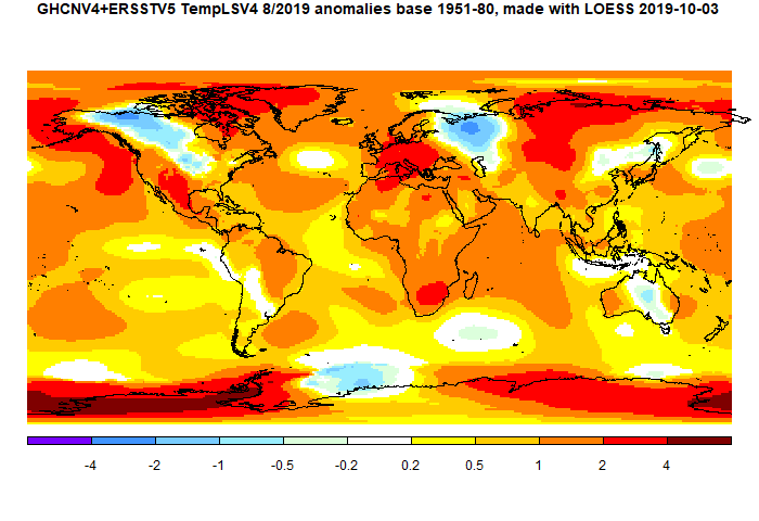
Tuesday, September 3, 2019
August NCEP/NCAR global surface anomaly up 0.017°C from July
The Moyhu NCEP/NCAR index rose from 0.372°C in July to 0.389°C in August, on a 1994-2013 anomaly base. Like the last two months, it was uneventful but globally quite warm.
NW Canada down into the US midwest was cool. E Siberia was warm, but W Russia was cool. The extremes were around Antarctica, with parts of the adjacent ocean being very cool, but warm areas on land, especially W Antarctica. Australia was cool.
NW Canada down into the US midwest was cool. E Siberia was warm, but W Russia was cool. The extremes were around Antarctica, with parts of the adjacent ocean being very cool, but warm areas on land, especially W Antarctica. Australia was cool.
Friday, August 30, 2019
Mapping projections for climate data
When I first planned to post sets of climate data, usually temperature, as color maps, I thought about what kind of projection to use. There is some general discussion here. I decided to mostly settle for simple lat/lon or equirectangular plotting for routine use, but making use of Javascript active facilities to present an actual sphere (simply projected on the screen) where better geometry was needed. I first used a small set of views which the user could switch between, and then a HTML 5 version in which the user could choose an arbitrary view of the sphere by clicking on a small map. Then I moved on to WebGL globes which could be dragged by mouse. This has been further developed using a general WebGL facility which simplifies coding and data input and gives useful default capabilities. Incidentally, I still find the key map a useful way of controlling the globe.
But I have come back to thinking about plane projections. One reason is that I post images on Twitter, where I can't use Javascript. Another is that I compare TempLS output with GISS and other indices, and often their default presentation is with some other projection. So I have looked at schemes such as Mollweide and Robinson, the latter being used by GISS and others.
This has linked in with another aspect of what I do, which is using Platonic solids as a basis for gridding for integration of temperature, and perhaps for graphics. As a by-product, I showed some equal area projections based on the cubed sphere. I have recently been using icosahedral grids in the same way, and that yields equal area maps with even less distortion, but which are also particularly informative for these applications.
So in this post I want to touch on some of these points. First the conventional projections.
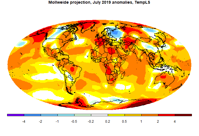
I am not a fan of the Robinson projection. It is billed as a compromise, but I think it is thus neither fish nor fowl. It is not much closer to equal area than lat/lon, and it does little to reduce distortion. It seems to be popular because it seems not unfamiliar to people used to equirectangular. However, it should be easy to implement, so there is little to lose by using it. I say should be, but in fact they make a considerable rigmarole, presenting a table of numbers to be used, and even fussing about how to interpolate. This may be because there are still ownership issues, although there seem to be no restrictions on use. Anyway, I'll describe my way of implementing in the appendix.
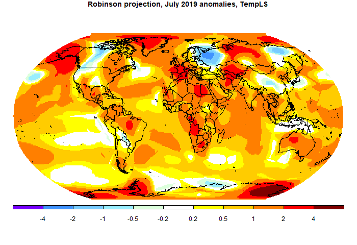
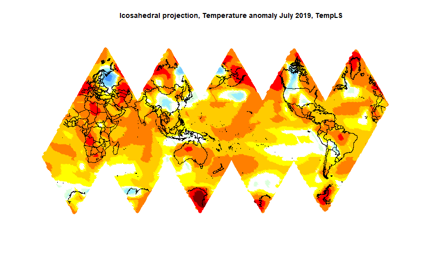
It is very close to equal area. This is achieved at the expense of more numerous cuts. It is not so easy to figure out, and may not be the best projection for this purpose. But it is more useful for showing the distribution of stations, where area density is more critical. I'm using it to see reasons for possible failure of an integration scheme based on icosahedra. Here is the plot:
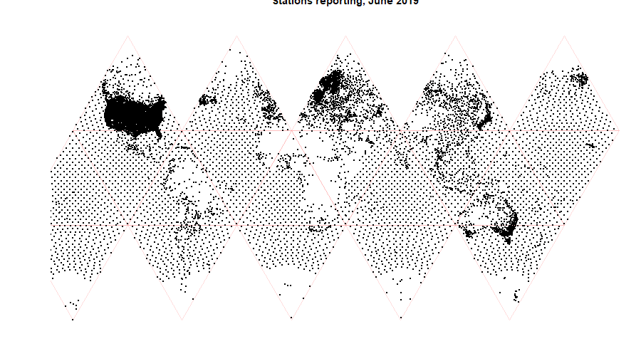
Both the Mollweide and Robinson projections have a similar simple basis. There is one mapping of latitudes from old to new, and then a formula for scaling the longitudes. Latitudes remain as horizontal lines. So two functions of a single variable (each) need to be approximated. There is a little difficulty with singularity in the Mollweide.
In each case, the latitude transform is an odd function (about zero latitude), and the longitude scale is even. I require the approximation to be exact at the equator and poles, and a least squares fit elsewhere. So generally, if the original coordinates are (x,y), x=longitude, angles in right angle units, and the projection coords are (X,Y), the mapping is
Y=f(y)=y+y(1-y²)(a₀ +a₁y² +a₂y4 +...)
X=x*g(y); g(y)=1-d*y²+y²(1-y²)(b₀ +b₁y² +b₂y4 +...)
The inverses are
y=F(Y)=Y+Y(1-Y²)(c₀ +c₁Y² +c₂Y4 +...)
x=X/g(y)
For the Robinson projection I find the coefficients by fitting to the data tabulated by Wiki. d is just what is needed to get X right at y=1, so = 1-X there. From the table, that is d = 1-0.5322 = 0.4678.
The coefficients are, to four terms:
The Mollweide formula relates f(y) in terms of an intermediate variable a :
Y=sin(a)
2a+sin(2a)=π sin(π/2 y)}}
So I generate a sequence of values of a between 0 and π/2, and hence y and Y sequences that I can use for fitting, to get f and F. But first there is a wrinkle near y=1; the expansion of the second equation there relates (1-a)³ on the left to (1-y)², and it is necessary to take fractional powers. The simplest thing to do is to first transform
z=sqrt(1-(1-y²)^(4/3))
and then do the expansion in z. Then it is necessary to map back again
Y=sqrt(1-(1-z²)^(3/4))
However, a simplification is now that the function g(y) is just sqrt(1-y²). And d=1. So the series are:
a:(0.06818,0.01282,-0.01077,0.01949)
c: (-0.06395,-0.0142,0.00135,-0.0085)
All these approximations give considerably better than three sig fig accuracy, which means error much less than a pixel.
But I have come back to thinking about plane projections. One reason is that I post images on Twitter, where I can't use Javascript. Another is that I compare TempLS output with GISS and other indices, and often their default presentation is with some other projection. So I have looked at schemes such as Mollweide and Robinson, the latter being used by GISS and others.
This has linked in with another aspect of what I do, which is using Platonic solids as a basis for gridding for integration of temperature, and perhaps for graphics. As a by-product, I showed some equal area projections based on the cubed sphere. I have recently been using icosahedral grids in the same way, and that yields equal area maps with even less distortion, but which are also particularly informative for these applications.
So in this post I want to touch on some of these points. First the conventional projections.
Mollweide and Robinson
These are of course well-established. But I found the Wiki versions of the implementation unnecessarily hard to implement, so I'll describe in an appendix some simple approximating formulae. The Mollweide projection achieves equal area at a cost of some distortion near poles. Equal area can be desirable, as for example in not exaggerating the weather variations near poles. One particular use I will describe is in displaying the extent of coverage of temperature stations. Here is a typical map:I am not a fan of the Robinson projection. It is billed as a compromise, but I think it is thus neither fish nor fowl. It is not much closer to equal area than lat/lon, and it does little to reduce distortion. It seems to be popular because it seems not unfamiliar to people used to equirectangular. However, it should be easy to implement, so there is little to lose by using it. I say should be, but in fact they make a considerable rigmarole, presenting a table of numbers to be used, and even fussing about how to interpolate. This may be because there are still ownership issues, although there seem to be no restrictions on use. Anyway, I'll describe my way of implementing in the appendix.
Icosahedral projection
I'm developing yet another method of integration, based on FEM on an icosahedral mesh. I'll post soon. But meanwhile it makes for an interesting projection.It is very close to equal area. This is achieved at the expense of more numerous cuts. It is not so easy to figure out, and may not be the best projection for this purpose. But it is more useful for showing the distribution of stations, where area density is more critical. I'm using it to see reasons for possible failure of an integration scheme based on icosahedra. Here is the plot:
What next?
I'll try using the Robinson projection for the regular TempLS reports, mainly to make it easier to compare with others. I'll probably also occasionally show a Mollweide projection.Appendix - calculation methods
As I mentioned, I found the Wiki versions surprisingly clunky, so I spent some time developing simpler ways. I need that partly because I have to be able to reverse. When I show a color plot, I need to define a grid of points on the projection, map back to the sphere for interpolation, and then bring the colors back.Both the Mollweide and Robinson projections have a similar simple basis. There is one mapping of latitudes from old to new, and then a formula for scaling the longitudes. Latitudes remain as horizontal lines. So two functions of a single variable (each) need to be approximated. There is a little difficulty with singularity in the Mollweide.
In each case, the latitude transform is an odd function (about zero latitude), and the longitude scale is even. I require the approximation to be exact at the equator and poles, and a least squares fit elsewhere. So generally, if the original coordinates are (x,y), x=longitude, angles in right angle units, and the projection coords are (X,Y), the mapping is
Y=f(y)=y+y(1-y²)(a₀ +a₁y² +a₂y4 +...)
X=x*g(y); g(y)=1-d*y²+y²(1-y²)(b₀ +b₁y² +b₂y4 +...)
The inverses are
y=F(Y)=Y+Y(1-Y²)(c₀ +c₁Y² +c₂Y4 +...)
x=X/g(y)
For the Robinson projection I find the coefficients by fitting to the data tabulated by Wiki. d is just what is needed to get X right at y=1, so = 1-X there. From the table, that is d = 1-0.5322 = 0.4678.
The coefficients are, to four terms:
| a: | 0.1123 | 0.1890 | -0.1722 | 0.2326 |
| b: | -0.0885 | -0.3568 | 0.8331 | -1.0023 |
| c: | 0.1782 | -0.6687 | 1.1220 | -0.8133 |
The Mollweide formula relates f(y) in terms of an intermediate variable a :
Y=sin(a)
2a+sin(2a)=π sin(π/2 y)}}
So I generate a sequence of values of a between 0 and π/2, and hence y and Y sequences that I can use for fitting, to get f and F. But first there is a wrinkle near y=1; the expansion of the second equation there relates (1-a)³ on the left to (1-y)², and it is necessary to take fractional powers. The simplest thing to do is to first transform
z=sqrt(1-(1-y²)^(4/3))
and then do the expansion in z. Then it is necessary to map back again
Y=sqrt(1-(1-z²)^(3/4))
However, a simplification is now that the function g(y) is just sqrt(1-y²). And d=1. So the series are:
a:(0.06818,0.01282,-0.01077,0.01949)
c: (-0.06395,-0.0142,0.00135,-0.0085)
All these approximations give considerably better than three sig fig accuracy, which means error much less than a pixel.
Friday, August 16, 2019
GISS July global up 0.01°C from June.
The GISS V4 land/ocean temperature anomaly rose 0.01°C in July. The anomaly average was 0.93°C, up from June 0.92°C. It compared with a 0.061°C rise in TempLS V4 mesh I originally posted a 0.33°C rise, but this drifted upward with late data). As with TempLS, it was the warmest July in the GISS record, also by a considerable margin (0.08°C warmer than 2016).
The overall pattern was similar to that in TempLS. Hot in Africa and most of Europe, extending into Central Asia. Cool in NW Russia. Coolish in much of N America, but warm in Alaska, extending across Bering Strait. Warm in Greenland, mixed in Antarctica.
As usual here, I will compare the GISS and earlier TempLS plots below the jump.
Friday, August 9, 2019
Active WebGL plot of decadal regional temperature trends using ERSST V5 and GHCN V4
I have maintained a page of local trends over periods that users could choose. It was based on GHCN V3, and mesh display, and can still be seen here. But I need to upgrade to GHCN V4, and I have decided to update to LOESS graphics as well. But there is one further upgrade - instead of a choice of a fixed number of intervals ending in present, you can now choose any period of decades back to 1900. The maths of this is quite interesting, and I'll say more below. The new page is here, with the link in the page list top right.
The plot itself is the usual WebGL trackball. You can drag the globe around, or more quickly relocate by clicking on the small map above. Clicking on the plot shows the trend for the chosen period at that location. You can choose periods with the buttons on the right. The endpoints are colored, so the start state of 1980 and 2020 means the period will be Jan 1980 to Dec 2019, with missing months suitably handled. If you click outside the range, the range will extend; if you click inside, the red color will move to your choice. If you wanted to move the pink end, click the pink button to make it red. When you have chosen, click the Show button at the top to get the new plot. The average global trend for the period will show at the bottom as well.
The plot itself is the usual WebGL trackball. You can drag the globe around, or more quickly relocate by clicking on the small map above. Clicking on the plot shows the trend for the chosen period at that location. You can choose periods with the buttons on the right. The endpoints are colored, so the start state of 1980 and 2020 means the period will be Jan 1980 to Dec 2019, with missing months suitably handled. If you click outside the range, the range will extend; if you click inside, the red color will move to your choice. If you wanted to move the pink end, click the pink button to make it red. When you have chosen, click the Show button at the top to get the new plot. The average global trend for the period will show at the bottom as well.
Methods
As usual, the sphere is a trackball that you drag into position, or you can quickly set by clicking on the small map at the top. Beside that map are checkboxes which let you switch the objects displayed. The icosahedral mesh and nodes are initially not shown.The map is created by first getting monthly averages on the 5762 icosahedral nodes, as described here and here. The trends are then calculated on those nodes. The LOESS method takes a weighted local linear regression on the closest station/SST data, even if it is not close at all. In Antarctica, for example, before 1960 that generally means ocean data. So trends for Antarctica for early times should be ignored. Elsewhere, there is loss of resolution according to station data, but it is still reasonably based. GHCN V4, of course, has much better coverage than V3.
Note that the color scheme is centered for zero trend, but the range varies with the length of period.
Discussion
I think there is a lot to learn from the graphic, and I'll write a more detailed post. For example, recent periods show the extent to which warming dominates the Arctic, but if you look at the most recent decade, it's more mixed, with pronounced cooling over Greenland and the Canadian islands, but warming around Bering Strait. In earlier periods The warming extends to N Siberia as well.It's interesting to look at the period 1910-1940, often used by skeptics to say that AGW is refute. It's often accompanied by a whinge about how that warming is being suppressed, often showing a plot of Hansen in 1981 or NCAR in 1974 to claim that their warming has been watered down since.
But this plot shows what was happening. Again Arctic warming dominates, and to a lesser extent, N America and N Atlantic. But the S Hemisphere and most oceans show very little warming. Those earlier plots were land only, with data heavily weighted to the N Hemisphere. The reduced warming in later calculations have the advantage of this knowledge.
I originally started out here to do a corresponding plot of the differences between GHCN V3 and V4, and that will be an upcoming post. It is working - just a little more checking.
Trend methods
I'll just say a little about the data handling here. I try to keep the volume of data down; not so much for my web storage, but because of download time. So I used moments. The zero'th moment of numbers yₖ with location is just the sum. The first central moment is the sum Σ(k-kₒ)yₖ, where kₒ is trhe mean. And the trend is just the first central moment, normalised by division by the moment of a unit trend.There is a trick with moments familiar from calculating angular momentum, say. To get the moment of some bodies, you can just add the moments of their masses (zeroth moments) at their centres of mass, and add in the central first moments of each body. So here, I can just calculate and transmit the zero'th and first moments of the decades, and then I can work out the trend for any sequence of decades.
Tuesday, August 6, 2019
July global surface TempLS up 0.033°C from June.
The TempLS mesh anomaly (1961-90 base) was 0.813deg;C in July vs 0.78°C in June. This is a little more than the 0.018°C rise in the NCEP/NCAR reanalysis base index.
In contrast to the reanalysis, though, it did make it the warmest July in the record, and by a significant margin - 0.744°C in 2016 was next. The prospect of July being warmest has started a number of "hottest month ever" stories. I don't join in that, because it is only true if you add the seasonal cycle that makes NH summer the global peak. There are good reasons why we quote anomalies rather than absolute temperatures, so deviating for this claim can only cause confusion. In any case the seasonal cycle is predictable; the news is the anomaly. And July was nowhere near the highest anomaly of all months. Last March, for example, was 0.982°C.
Interestingly, the increase was due mostly to an SST rise, as was last month. Rising SST tends to continue for longer periods. On land, Much of North America was cool, except Alaska, and some of E Canada. S Europe was warm, but there was a cool spot in NW Russia. There was a warm band through central Asia to Iran and on to the Sahara. Antarctica was mostly warm.
Update 15 Aug Readers following the TempLS report may have noticed some unexpected variations in the July average. About 4 days ago the mesh version dropped to about the June level, and more seriously, the SST dropped back. TempLS LOESS was unaffected, as were the maps and graphics. The reason was that I had been tinkering with the cross product library routine that the mesh area weighting uses. I have fixed that, and now the surprise is that August is now 0.061°C warmer that July, rather than the posted 0.033°C. But I think that is genuine - it had been drifting higher before the sudden drop.
I'll show the bar chart of contributions; these are basically temperatures weighted by area. Africa and Antarctica were most responsible for the rise.
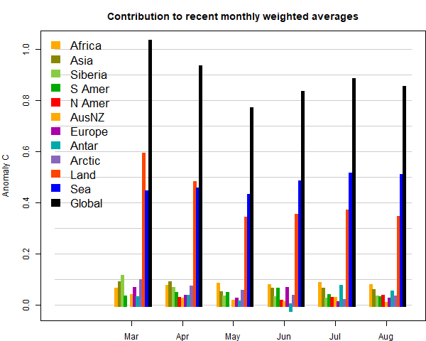
Here is the temperature map, using the LOESS-based map of anomalies.
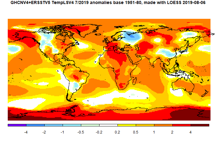
In contrast to the reanalysis, though, it did make it the warmest July in the record, and by a significant margin - 0.744°C in 2016 was next. The prospect of July being warmest has started a number of "hottest month ever" stories. I don't join in that, because it is only true if you add the seasonal cycle that makes NH summer the global peak. There are good reasons why we quote anomalies rather than absolute temperatures, so deviating for this claim can only cause confusion. In any case the seasonal cycle is predictable; the news is the anomaly. And July was nowhere near the highest anomaly of all months. Last March, for example, was 0.982°C.
Interestingly, the increase was due mostly to an SST rise, as was last month. Rising SST tends to continue for longer periods. On land, Much of North America was cool, except Alaska, and some of E Canada. S Europe was warm, but there was a cool spot in NW Russia. There was a warm band through central Asia to Iran and on to the Sahara. Antarctica was mostly warm.
Update 15 Aug Readers following the TempLS report may have noticed some unexpected variations in the July average. About 4 days ago the mesh version dropped to about the June level, and more seriously, the SST dropped back. TempLS LOESS was unaffected, as were the maps and graphics. The reason was that I had been tinkering with the cross product library routine that the mesh area weighting uses. I have fixed that, and now the surprise is that August is now 0.061°C warmer that July, rather than the posted 0.033°C. But I think that is genuine - it had been drifting higher before the sudden drop.
I'll show the bar chart of contributions; these are basically temperatures weighted by area. Africa and Antarctica were most responsible for the rise.
Here is the temperature map, using the LOESS-based map of anomalies.
Saturday, August 3, 2019
July NCEP/NCAR global surface anomaly up 0.018°C from June
The Moyhu NCEP/NCAR index rose from 0.354°C in June to 0.372°C in July, on a 1994-2013 anomaly base. This index fell last month when most others rose, so it remains on the cool side. While there is much talk of July being the hottest ever, allowing for the seasonal cycle, in this NCEP/NCAR index it was behind 2016 at 0.414°C.
North America was mostly cool, except Alaska. S Europe was warm, but E Europe and W Russia were cool. There was a warm band through central Asia to Iran. Antarctica had both very warm and very cool patches, the cool being mostly ocean.
North America was mostly cool, except Alaska. S Europe was warm, but E Europe and W Russia were cool. There was a warm band through central Asia to Iran. Antarctica had both very warm and very cool patches, the cool being mostly ocean.
Thursday, August 1, 2019
Unadjusted GHCN V3 and V4 global differences due to coverage, not content.
In yesterday's post I did a graphical study of the differences of GHCN V3 and V4 anomalies for June 2019. The idea was to try to pin down what caused a small discrepancy in the global average for that month. Clive Best has been looking at this, and thinks there may be a systematic change in reported temperatures between versions. My conclusion was that the difference was not because V4 was reporting higher temperatures, but that the greater coverage fixed a problem in V3 that in sparsely covered areas, sea temperatures would have an influence on land. I should add that this is a potential problem in TempLS and in Clive's similar code based on triangle mesh. I think these are very good methods, but the main codes do have one feature that they process land and sea separately, which should reduce this effect.
Clive sought to establish a link by finding a common set of V3 and V4, and seeing whether the difference persisted. I wasn't sure of this, because while there may be a common inventory, the stations in any one month won't correspond. I proposed a test in which the locations of GHCN V3 stations reporting in a month would have values interpolated (by mesh) from the V4 result. But they would then be analysed using the V3 mesh. I suspected that the result would be closer to V3 than V4, which would indicate that the difference was due to the reduced coverage, rather than a discrepancy between the temperature levels of the measures.
I'm reporting on that here. To summarise what I did - I had results from a run of the mesh method for both V3 and V4, reported here. From the V4 directory, I copied the node locations Z4, the anomalies A4, the weights W4, and I rebuilt the mesh M4. TempLS does integration by calculating weights, so the global average is the scalar product W4.A4. From the V3 directory, I copied the locations Z3 and weights W3. Then I linearly interpolated A4 onto Z3, using the mesh M4, giving result Aa. The "hybrid average" is then the scalar product W3.Aa, and it is being compared with W4.A4 and W3.A3.
So here is the first plot. I am presenting them as difference plots, because, as you can see from the plots here, the differences are small and hard to see against the full range of variation of the anomalies. Here is a plot of the last 30 months, with unadjusted data.
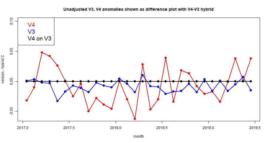
The V4 plot seems to jump around more, and clearly the V3 plot is a better match. In reality, the V3 anomaly fluctuates just as much as V4, if not more, but the hybrid tracks better with V3. I'll show another plot of the last 60 Junes:
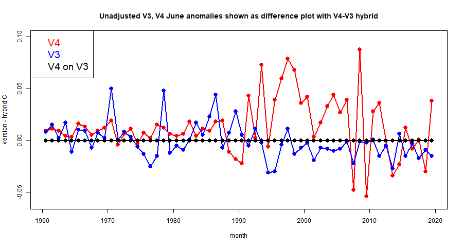
There are more interesting features here. back to about 1990, the hybrid fairly closely tracks V3, with quite a lot of variability between V3 and V4, mostly with V4 warmer. But before 1990 V4 calms down, and only occasional spurts from V3, now not tracked by the hybrid. It's hard to know what to make of this; except for V3 excursions, both V4 and V3 seem in agreement with the hybrid, and so with each other.
The story is slightly different with adjusted data, V3 and v4. Here is the plot of the last 30 months:
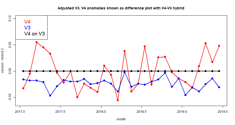
The V3 difference still jumps around a lot less, but there is a fairly persistent offset of up to 0.02°F. This might reasonably be attributed to an effect of homogenisation. Finally, here are the adjusted data averages differenced over the last 60 Junes.
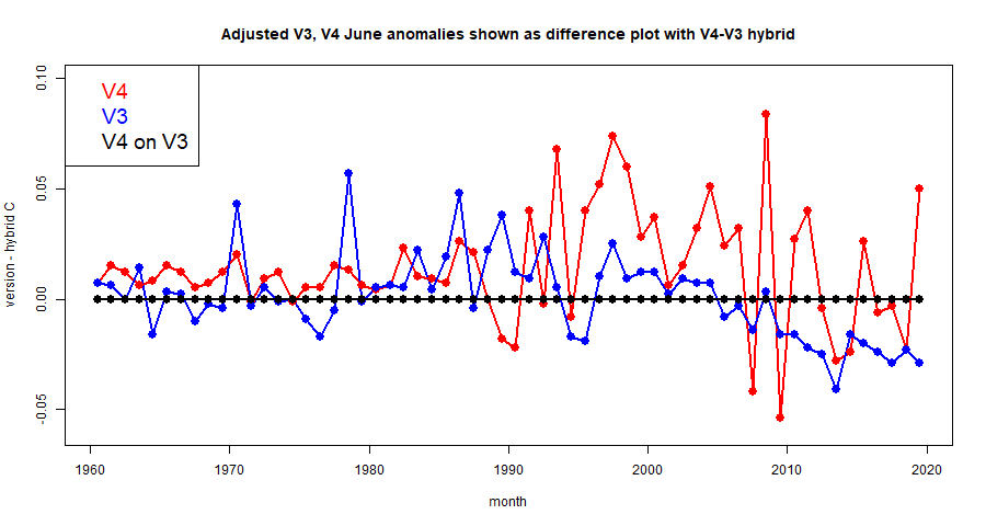
The adjusted pattern reflects the same interesting features as the unadjusted, with big differences between V4 and V3, and the hybrid mostly tracking V3, but with a departure during the last decade. Before 1990, less variation generally, with no obvious tendency for the hybrid to preferentially track V3.
The purpose of this post was to give some quantitative backing to the effects on the average that might be expected from the patterns shown in the last post. The adherence of the unadjusted data hybrid to v3 does not support the idea that there is a recent decades bias in the V4 measured data relative to V3. The performance of adjusted data does suggest a small effect arising from the V4 data, with some rather interesting behaviour going back before 1990 (for Junes).
Clive sought to establish a link by finding a common set of V3 and V4, and seeing whether the difference persisted. I wasn't sure of this, because while there may be a common inventory, the stations in any one month won't correspond. I proposed a test in which the locations of GHCN V3 stations reporting in a month would have values interpolated (by mesh) from the V4 result. But they would then be analysed using the V3 mesh. I suspected that the result would be closer to V3 than V4, which would indicate that the difference was due to the reduced coverage, rather than a discrepancy between the temperature levels of the measures.
I'm reporting on that here. To summarise what I did - I had results from a run of the mesh method for both V3 and V4, reported here. From the V4 directory, I copied the node locations Z4, the anomalies A4, the weights W4, and I rebuilt the mesh M4. TempLS does integration by calculating weights, so the global average is the scalar product W4.A4. From the V3 directory, I copied the locations Z3 and weights W3. Then I linearly interpolated A4 onto Z3, using the mesh M4, giving result Aa. The "hybrid average" is then the scalar product W3.Aa, and it is being compared with W4.A4 and W3.A3.
So here is the first plot. I am presenting them as difference plots, because, as you can see from the plots here, the differences are small and hard to see against the full range of variation of the anomalies. Here is a plot of the last 30 months, with unadjusted data.
The V4 plot seems to jump around more, and clearly the V3 plot is a better match. In reality, the V3 anomaly fluctuates just as much as V4, if not more, but the hybrid tracks better with V3. I'll show another plot of the last 60 Junes:
There are more interesting features here. back to about 1990, the hybrid fairly closely tracks V3, with quite a lot of variability between V3 and V4, mostly with V4 warmer. But before 1990 V4 calms down, and only occasional spurts from V3, now not tracked by the hybrid. It's hard to know what to make of this; except for V3 excursions, both V4 and V3 seem in agreement with the hybrid, and so with each other.
The story is slightly different with adjusted data, V3 and v4. Here is the plot of the last 30 months:
The V3 difference still jumps around a lot less, but there is a fairly persistent offset of up to 0.02°F. This might reasonably be attributed to an effect of homogenisation. Finally, here are the adjusted data averages differenced over the last 60 Junes.
The adjusted pattern reflects the same interesting features as the unadjusted, with big differences between V4 and V3, and the hybrid mostly tracking V3, but with a departure during the last decade. Before 1990, less variation generally, with no obvious tendency for the hybrid to preferentially track V3.
The purpose of this post was to give some quantitative backing to the effects on the average that might be expected from the patterns shown in the last post. The adherence of the unadjusted data hybrid to v3 does not support the idea that there is a recent decades bias in the V4 measured data relative to V3. The performance of adjusted data does suggest a small effect arising from the V4 data, with some rather interesting behaviour going back before 1990 (for Junes).
Subscribe to:
Posts (Atom)


