Methods of integrating temperature anomalies on the sphere

A few days ago, I described a new method for integrating temperature anomalies on the globe, which I called FEM/LOESS. I think it may be the best general purpose method so far. In this post I would like to show how well it works within TempLS, with comparisons with other advanced methods. But first I would like to say a bit more about the mathematics of the method. I'll color it blue for those who would like to skip.

Mathematics of FEM/LOESS

It's actually a true hybrid of the finite element method (FEM) and LOESS (locally estimated scatterplot smoothing). In LOESS a model is fitted locally by regression, usually to get a central value. In FEM/LOESS, the following least squares parameter fit is made:

The standard FEM approximate function is f(z)=ΣaᵢBᵢ(z) where z is location on the sphere, B are the basis functions described in the previous post, and aᵢ are the set of coefficients to be found by fitting to a set of observations that I will call y(z). The LS target is

SS=∫(f(z)-y(z))^2 dz

This has to be estimated knowing y at a discrete points (stations). In FEM style, the integral is split into integrals over elements, and then within elements the integrand is estimated as mean (f(zₖ)-y(zₖ))^2 over points k. One might question whether the sum within elements should be weighted, but the idea is that the fitted f() takes out the systematic variation, so the residuals should be homogeneous, and a uniform mean is correct.

So differentiating wrt a to minimise:
∫(f(z)-y(z))Bᵢ(z) dz = 0
Discretising:

Σₘ Eₘ (ΣₖBᵢ(zₖ)Bₙ(zₖ)aₙ)/(Σₖ1) = Σₘ Eₘ (ΣₖBᵢ(zₖ)yₖ)/(Σₖ1)

The first summation is over elements, and E are their areas. In FEM style, the summations that follow are specific to each element, and for each E include just the points zₖ within that element, and so the basis functions in the sum are those that have a node within or on the boundary if that element. The denominators Σₖ1 are just the count of points within each element. It looks complicated but putting it together is just the standard FEM step of assembling a mass matrix.

In symbols,this is the regression equation
H a = B^* w B a = B^* w y
where B is the matrix of basis functions evaluated at zₖ, B^* transpose, diagonal matrix w the weights Σₘ/(Σₖ1) (area/count), y the vector of readings, and a the vector of unknown coefficients.

To integrate a specific y, this has to be solved for a:
a=H^-1B^* w y
and then ΣaᵢBᵢ(z) integrated on the globe
Int = ΣaᵢIᵢ where Iᵢ is the integral of function Bᵢ,

H is generally positive definite and sparse, so the inversion is done with conjugate gradients, using the diagonal as preconditioner.

For TempLS I need not an integral but weights. So I have to calculate

wt = I H^-1B^* w

It sounds hard, but it is a well trodden FEM task, and is computationally quite fast. In all this a small multiple of a Laplacian matrix is added to H to ensure corresponding infilling of empty or inadequately constrained cells.

Comparisons

I ran TempLS using the FEM/LOESS weighting with 9 modes, h2p2, h2p3, h2p4,...h43,h4p4. I calculated the RMS of differences between monthly averages, pairwise, for the years 1900-2019, and similar differences between and within the advanced methods MESH, LOESS and INFILL (see here for discussion, and explanation of the h..p.. notation). Here is a table of results, of RMS difference in °C, multiplied by 1000:

	MESH	LOESS	INFILL	h2p2	h3p2	h4p2	h5p2	h2p3	h3p3	h4p3	h5p3	h2p4	h3p4	h4p4	h5p4	h2p5	h3p5	h4p5	h5p5
MESH	0	18	19	26	20	19	19	21	18	17	19	18	17	17	19	19	19	19	22
LOESS	18	0	25	24	22	19	22	20	22	20	23	19	22	21	24	22	23	24	27
INFILL	19	25	0	27	19	17	14	21	14	13	11	17	11	11	10	14	11	10	12
h2p2	26	24	27	0	24	25	26	21	24	24	26	22	25	25	26	26	26	27	28
h3p2	20	22	19	24	0	17	16	16	11	16	17	16	12	17	18	16	17	17	21
h4p2	19	19	17	25	17	0	14	15	12	8	16	12	13	10	14	14	16	17	20
h5p2	19	22	14	26	16	14	0	17	11	11	6	13	10	10	12	0	6	8	12
h2p3	21	20	21	21	16	15	17	0	16	16	19	10	17	17	19	17	19	20	23
h3p3	18	22	14	24	11	12	11	16	0	10	11	12	6	10	12	11	11	13	16
h4p3	17	20	13	24	16	8	11	16	10	0	11	11	9	4	9	11	11	12	16
h5p3	19	23	11	26	17	16	6	19	11	11	0	15	9	9	10	6	0	4	8
h2p4	18	19	17	22	16	12	13	10	12	11	15	0	13	12	15	13	15	16	20
h3p4	17	22	11	25	12	13	10	17	6	9	9	13	0	8	10	10	9	10	14
h4p4	17	21	11	25	17	10	10	17	10	4	9	12	8	0	6	10	9	10	14
h5p4	19	24	10	26	18	14	12	19	12	9	10	15	10	6	0	12	10	9	12
h2p5	19	22	14	26	16	14	0	17	11	11	6	13	10	10	12	0	6	8	12
h3p5	19	23	11	26	17	16	6	19	11	11	0	15	9	9	10	6	0	4	8
h4p5	19	24	10	27	17	17	8	20	13	12	4	16	10	10	9	8	4	0	6
h5p5	22	27	12	28	21	20	12	23	16	16	8	20	14	14	12	12	8	6	0

The best agreement between the older methods is between MESH and LOESS at 18. Agreement between the higher order FEM results is much better. Agreement of FEM with MESH is a little better, with LOESS a little worse. The agreement with INFILL is better again, but needs to be discounted somewhat. The reason is that in earlier years there is a large S Pole region without data. Both INFILL and FEM deal with this with Laplace interpolation, so I think that spuriously enhances the agreement.
As will be seen later, there is a change in the matchings at about 1960, when Antarctic data becomes available. So I did a similar table just for the years since 1960:

	MESH	LOESS	INFILL	h2p2	h3p2	h4p2	h5p2	h2p3	h3p3	h4p3	h5p3	h2p4	h3p4	h4p4	h5p4	h2p5	h3p5	h4p5	h5p5
MESH	0	11	11	23	17	16	14	18	13	12	12	15	12	11	10	14	12	12	16
LOESS	11	0	10	19	14	12	10	14	10	9	9	10	9	8	9	10	9	10	14
INFILL	11	10	0	21	16	16	13	17	13	12	11	15	11	10	9	13	11	10	13
h2p2	23	19	21	0	20	20	20	18	20	20	20	18	20	20	21	20	20	20	22
h3p2	17	14	16	20	0	15	15	13	10	14	15	13	11	14	16	15	15	15	19
h4p2	16	12	16	20	15	0	12	12	10	7	14	9	10	9	13	12	14	16	20
h5p2	14	10	13	20	15	12	0	15	11	9	6	11	10	10	11	0	6	8	13
h2p3	18	14	17	18	13	12	15	0	12	13	16	10	13	14	16	15	16	17	20
h3p3	13	10	13	20	10	10	11	12	0	9	12	8	6	9	11	11	12	13	17
h4p3	12	9	12	20	14	7	9	13	9	0	10	9	7	4	8	9	10	11	16
h5p3	12	9	11	20	15	14	6	16	12	10	0	13	9	9	9	6	0	4	9
h2p4	15	10	15	18	13	9	11	10	8	9	13	0	9	9	12	11	13	14	18
h3p4	12	9	11	20	11	10	10	13	6	7	9	9	0	7	9	10	9	11	15
h4p4	11	8	10	20	14	9	10	14	9	4	9	9	7	0	6	10	9	10	15
h5p4	10	9	9	21	16	13	11	16	11	8	9	12	9	6	0	11	9	9	13
h2p5	14	10	13	20	15	12	0	15	11	9	6	11	10	10	11	0	6	8	13
h3p5	12	9	11	20	15	14	6	16	12	10	0	13	9	9	9	6	0	4	9
h4p5	12	10	10	20	15	16	8	17	13	11	4	14	11	10	9	8	4	0	7
h5p5	16	14	13	22	19	20	13	20	17	16	9	18	15	15	13	13	9	7	0

Clearly the agreement is much better. The best of the older methods is between LOESS and INFILL at 10. But agreement between high order FEM methods is better. Now it is LOESS that agrees well with FEM - better than the others. Of course in assessing agreement, we don't know which is right. It is possible that FEM is the best, but not sure.

Here are some time series graphs. I'll show a time series graph first, but the solutions are too close to distinguish much.





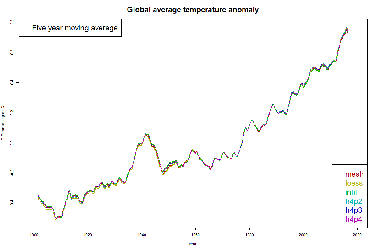
Difference plots are more informative. These are made by subtracting one of the solutions from the others. I have made plots using each of MESH, LOESS and INFILL as reference. You can click the buttons below the plot to cycle through.



There is a region of notably good agreement between 1960 and 1990. This is artificial, because that is the anomaly base period, so all plots have mean zero there. Still, they are unusually aligned in slope.

Before 1960, LOESS deviates from the FEM curves, MESH less, and INFILL least. The agreement of INFILL probably comes from the common use of Laplace interpolation for the empty Antarctic region. In the post 1990 period, it is LOESS which best tracks with FEM.

However, I should note that no discrepancies exceed about 0.02°C.

Next steps

After further experience, I will probably make FEM/LOESS my frontline method.