Monday, March 25, 2019

Evenly spaced icosahedral grid for global temperature

I have been working on a new integration method for the next version of TempLS, V4. I call it the LOESS method; it works by local regression onto an evenly spaced set of nodes, where the anomalies can then be averaged. But the question then is, how to get that evenly spaced set of nodes.

I have written a lot about that before. The basic idea is to place points evenly on one of the five platonic solids, and then map them onto the sphere. The platonic solids are at least somewhat similar in shape to the sphere. I wrote here about using the cube (called a cubed sphere), and here with general ideas about gridding, with emphasis on the icosahedron .

A problem is that projection from the regular solid to the sphere does not preserve equal spacing. The central parts of the face are spread out by being projected further, while the areas near the vertices are actually compressed, since the face is inclined to the surface normal to the projection. For the cube, the area ratio is about 3:1; for the icosahedron it is about 2:1. In the cube post I explained a mapping that could be applied to the faces before projection, which would counter the disparity. I wrote here about how this could be applied to get an equal area projection (at the cost of cuts) for earth mapping.

I had some trouble extending this to the icosahedron, because I couldn't see a general mapping scheme with the right properties. But I now do see one based on homogeneous coordinates (also called projective or trilinear), which is simple and effective. I talk a bit about homogeneous coordinates, so I should digress to say a bit more about them. I'll put this digression in blue, so you can skip if you want.

Homogeneous coordinates

Every point x in a triangle is represented by three numbers (u1,u2,u3), which must add to 1. You can get x back, given the vertices (x1,x2,x3)
x = u1x1 + u2x2 + u3x3
and that illustrates an important role. They can interpolate properties known at the vertices by a similar formula. I'll make three points about them:

  1. The coordinates are often explained by areas. If you divided the triangle into three by connecting x to the vertices, then the proportion of area in the triangle opposite node 1 is its coordinate, etc.
  2. The coordinates are the real 3D coordinates of the equilateral triangle joining the unit points on the axes ((1,0,0), (0,1,0),(0,0,1)). The requirement to add to 1 is just the requirement that they lie on the plane through those 3 points. And since you can map those unit vertices onto the general triangle given by nodes (x1,x2,x3), you can map the interior points by multiplying by the same matrix. And it is the inverse of that matrix that takes an arbitrary triangle into the unit triangle. That is how you can calculate the homogeneous coordinates.
  3. The finite element method also has the idea of an interpolation, or basis, function. You multiply the nodal values by the values of the basis function at an interior point to get the interpolate. So homogeneous coords are just a special case of linear basis functions for one particular shape. That enables generalisation of the mapping idea I will explain.

Mapping for uniformity

A mapping before projection has some basic requirements:
  • It must keep points within the face.
  • It must comply with the symmetries of the face. The reason for this is that points on the edges will be mapped within each face that they belong to. Symmetry is needed so they do not get sent to different places.
A way of ensuring this is to apply a simple function of one variable to each projective coordinate, to make new interpolation functions. The function will have to be monotonic, and zero at zero (to keep boundary nodes on the boundary). And to comply with the requirement that the new coords add to 1, the result muct be normalised by dividing by the sum.

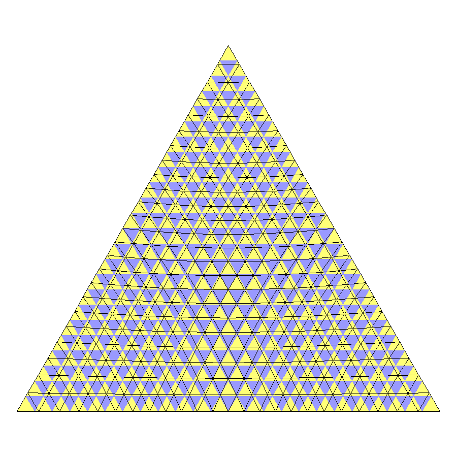
I chose a function of the form u/(1+a*u), because it is easily inverted (u/(1-a*u)). It is possible to determine a theoretically to make various match-ups, or just trial and error, since there is no perfect outcome. I found a value of 0.28 worked well. It means that instead of mapped triangles varying by a factor of 2, they only vary by 5%, which I think is good enough.

Here is a mapping of what is done. The icosahedron has 20 equilateral triangle faces. Each edge is divided into N equal parts. Connecting them with lines parallel to the edges makes N^2 with corresponding nodes. In this diagram, the purple triangles are the original regular grid, and the lines show the mapped grid. You'll see that the line triangles are larger near the corners, and smaller near the centre.

WebGL picture of the result

I used the WebGL facility to show the result on the sphere. In what follows, the sphere is a trackball that you can drag around. It's actually a LOESS plot of December 2018 temperatures, which I'll say more about in a future post. But in the style of the facility, you can use the checkboxes top right to hide various things. The mesh is clearer if you clear "mesh". make 'mesh_l" go away, and you can see the points better. You can dispense with the map too, if you want.


Tuesday, March 19, 2019

GISS February global up 0.05°C from January, third warmest February.

The GISS V3 land/ocean temperature anomaly rose 0.05°C in February. The anomaly average was 0.92°C, up from December 0.87°C. It compared with a 0.046°C rise in TempLS V3 mesh. I can't find Jim Hansen's monthly report on the web site, but his email linked to this page.

Like GISS, Moyhu is coming out with a V4 which will use GHCN V4. Actually, V3 could use it too, but it is time for a new version. GISS has marked theirs as beta - the monthly averages are here. V4 said the rise was only 0.01°C; Moyhu's V4 said the rise was higher, at 0.128°C. V4 of course has many more stations, and somewhat to my surprise, has xtensive reporting quite early; however, there is also extensive later data, and I'm still getting a feel for when it settles. My reporting is mixed; the main table shows V4, but the report and graphs are V3. This will change soon. I'll show below the anomaly maps for Moyhu and GISS V4 as well.

The overall pattern was similar to that in TempLS. W Canada and NW US were very cold, though SE US was quite warm.. Europe was warm, especially NE (Russia). Warmth also in Siberia and Alaska, and nearby Arctic. Australia was still quite warm. I'll note now that March so far is looking a whole lot warmer.

As usual here, I will compare the GISS and previous TempLS plots below the jump.

Sunday, March 10, 2019

February global surface TempLS (with GHCN V4) up 0.033°C from January.

TempLS is in transition from using GHCN V3 (which it has used for the last eight years) to the new GHCN V4. I'll report the V4 mesh results here, but for now, the Moyhu posted data is based on V3. I've been delayed a little because it is timely to also bring out a new version of TempLS (V4). Apart from anything else, the code needs reorganising to handle the bigger datasets smoothly. The Moyhu data page is still reporting values based on V3, as are the various pages with globe maps.

I worried about whether GHCN V4 would report as punctually as V3. But it seems to do better. Their version of 9 March showed 8779 stations reporting, compared with 10653 in January. But unlike V3, where countries report en bloc, here the reporting is spread, so no region is completely missing. I'll show a station map below.

TempLS mesh with V3 GHCN showed a larger rise, from 0.686°C to 0.779°C in February. This was more in line with the rise calculated with NCEP reanalysis. However, the V3 based infilled grid method was in agreement with V4 mesh, as was V4 infilled.

I'll write a post soon with a comparison of the whole V4-based history compared with V3. I'll also post a new version of TempLS which I have been using - I'll call that V4 too. It's mainly a restructuring to deal with the greater memory demands of GHCN V4, and also to include my new approach to handling spherical harmonics enhancement.

The TempLS mesh anomaly (1961-90 base) was 0.746deg;C in February vs 0.708°C in January. That makes it the third warmest February in the (V4-based) record.

The main feature of the month was rather severe cold over western Canada and adjacent US, but with warmth just a little to the North in the Arctic and Alaska. Europe was also very warm. There were patches of cool in the Sahara and western China.
Here is the temperature map.


And here is the map of land and sea stations reporting:


Monday, March 4, 2019

February NCEP/NCAR global surface anomaly up 0.097°C from January

The Moyhu NCEP/NCAR index rose from 0.296°C in January to 0.393°C in February, on a 1994-2013 anomaly base. That makes it the warmest month since May 2017. The warmth came mainly in a spurt at the end of the month, which is continuing.

It was quite cold in W Canada and the US, although warm in Alaska and the SE USA. Warm in Europe, cold in the Sahara, and mostly warm in Antarctica, with the Arctic mixed.

The BoM ENSO Outlook was is still set to Watch.