Another round of Pat Frank's "propagation of uncertainties.

See update below for a clear and important error.

There has been another round of the bizarre theories of Pat Frank, saying that he has found huge uncertainties in GCM outputs that no-one else can see. His paper has found a publisher - WUWT article here. It is a pinned article; they think it is a big deal.

The paper is in Frontiers or Earth Science. This is an open publishing system, with (mostly) named reviewers and editors. The supportive editor was Jing-Jia Luo, who has been at BoM but is now at Nanjing. The named reviewers are Carl Wunsch and Davide Zanchettin.

I wrote a Moyhu article on this nearly two years ago, and commented extensively on WUWT threads, eg here. My objections still apply. The paper is nuts. Pat Frank is one of the hardy band at WUWT who insist that taking a means of observations cannot improve the original measurement uncertainty. But he takes it further, as seen in the neighborhood of his Eq 2. He has a cloud cover error estimated annually over 20 years. He takes the average, which you might think was just a average of error. But no, he insists that if you average annual data, then the result is not in units of that data, but in units/year. There is a wacky WUWT to-and-fro on that beginning here. A referee had objected to changing the units of annual time series averaged data by inserting the /year. The referee probably thought he was just pointing out an error that would be promptly corrected. But no, he coped a tirade about his ignorance. And it's true that it is not a typo, but essential to the arithmetic. Having given it units/year, that makes it a rate that he accumulates. I vainly pointed out that if he had gathered the data monthly instead of annually, the average would be assigned units/month, not /year, and then the calculated error bars would be sqrt(12) times as wide.

One thing that seems newish is the emphasis on emulation. This is also a WUWT strand of thinking. You can devise simple time models, perhaps based on forcings, which will give similar results to GCMs for one particular variable, global averaged surface temperature anomaly. So, the logic goes, that must be what GCM's are doing (never mind all the other variables they handle). And Pat Frank's article has much of this. From the abstract: "An extensive series of demonstrations show that GCM air temperature projections are just linear extrapolations of fractional greenhouse gas (GHG) forcing." The conclusion starts: "This analysis has shown that the air temperature projections of advanced climate models are just linear extrapolations of fractional GHG forcing." Just totally untrue, of course, as anyone who actually understands GCMs would know.

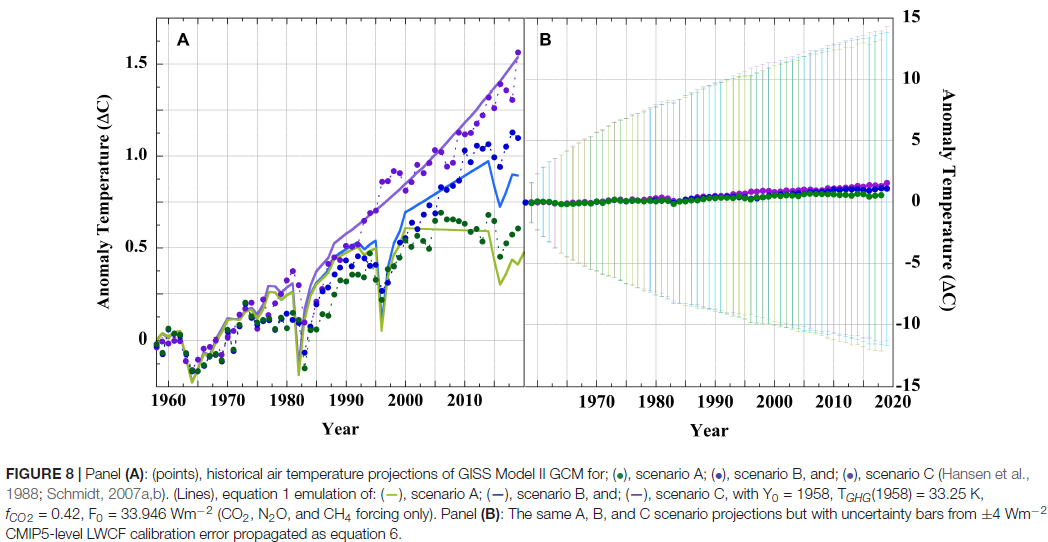
One funny thing - I pointed out here that PF's arithmetic would give a ±9°C error range in Hansen's prediction over 30 years. Now I argue that Hansen's prediction was good; some object that it was out by a small fraction of a degree. It would be an odd view that he was extraordinarily lucky to get such a good prediction with those uncertainties. But what do I see? This is now given, not as a reduction ad absurdum, but with a straight face as Fig 8:



To give a specific example of this nutty arithmetic, the paper deals with cloud cover uncertainty thus:

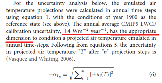
"On conversion of the above CMIP cloud RMS error (RMSE) as ±(cloud-cover unit) year^-1 model^-1 into a longwave cloud-forcing uncertainty statistic, the global LWCF calibration RMSE becomes ±Wm^-2 year^-1 model^-1. Lauer and Hamilton reported the CMIP5 models to produce an annual average LWCF root-mean-squared error (RMSE) = ±4 Wm^-2 year^-1 model^-1, relative to the observational cloud standard (81). This calibration error represents the average annual uncertainty within the simulated tropospheric thermal energy flux and is generally representative of CMIP5 models."

There is more detailed discussion of this starting here. In fact, Lauer and Hamilton said, correctly, that the RMSE was 4 Wm^-2. The year^-1 model^-1 is nonsense added by PF, but it has an important effect. The year^-1 translates directly into the amount of error claimed. If it had been month^-1, the claim would have been sqrt(12) higher. So why choose year? PF's only answer - because L&H chose to bin their data annually. That determines GCM uncertainty!

Actually, the ±4 is another issue, explored here. Who writes an RMS as ±4? It's positive. But again it isn't just a typo. An editor in his correspondence, James Annan wrote it as 4, and was blasted as an ignorant sod for omitting the ±. I pointed out that no-one, nor L&H in his reference, used a ± for RMS. It just isn't the meaning of the term. I challenged him to find that usage anywhere, with no result. Unlike the nutty units, I think this one doesn't affect the arithmetic. It's just an indication of being in a different world.

One final thing I should mention is the misunderstanding of climate models contained in the preamble. For example "Scientific models are held to the standard of mortal tests and successful predictions outside any calibration bound. The represented systems so derived and tested must evolve congruently with the real-world system if successful predictions are to be achieved."

But GCMs are models of the earth. They aim to have the same physical properties but are not expected to evolve congruently, just as they don't evolve congruently with each other. This was set out in the often misquoted IPCC statement

"In climate research and modelling, we should recognise that we are dealing with a coupled non-linear chaotic system, and therefore that the long-term prediction of future climate states is not possible. The most we can expect to achieve is the prediction of the probability distribution of the system’s future possible states by the generation of ensembles of model solutions. This reduces climate change to the discernment of significant differences in the statistics of such ensembles. "

Update - I thought I might just highlight this clear error resulting from the nuttiness of the /year attached to averaging. It's from p 12 of the paper:

Firstly, of course, they are not the dimensions (Wm^-2) given by the source, Lauer and Hamilton. But the dimensions don't work anyway. The sum of squares gives a year^-2 dimension component. Then just taking the sqrt brings that back to year^-1. But that is for the uncertainty of the whole period, so that can't be right. I assume Pat Frank puts his logic backward, saying that adding over 20 years multiplies the dimensions by year. But that still leaves the dimension (Wm^-2)² year^-1, and on taking sqrt, the unit is (Wm^-2)year^-1/2. Still makes no sense; the error for a fixed 20 year period should be Wm^-2.