How errors really propagate in differential equations (and GCMs).

There has been more activity on Pat Frank's paper since my last post. A long thread at WUWT, with many comments from me. And two good posts and threads at ATTP, here and here. In the latter he coded up Pat's simple form (paper here). Roy Spencer says he'll post a similar effort in the morning. So I thought writing something on how error really is propagated in differential equations would be timely. It's an absolutely core part of PDE algorithms, since it determines stability. And it isn't simple, but expresses important physics. Here is a TOC:

• Differential equations
• Fluids and Turbulence
• Error propagation
• GCM errors and conservation
• Simple equation analogies
• On Earth models
• Conclusion

Differential equations

An ordinary differential equation (de) system is a number of equations relating many variables and their derivatives. Generally the number of variables and equations is equal. There could be derivatives of higher order, but I'll restrict to one, so it is a first order system. Higher order systems can always be reduced to first order with extra variables and corresponding equations.

A partial differential equation system, as in a GCM, has derivatives in several variables, usually space and time. In computational fluid dynamics (CFD) of which GCMs are part, the space is gridded into cells or otherwise discretised, with variables associated with each cell, or maybe nodes. The system is stepped forward in time. At each stage there are a whole lot of spatial relations between the discretised variables, so it works like a time de with a huge number of cell variables and relations. That is for explicit solution, which is often used by large complex systems like GCMs. Implicit solutions stop to enforce the space relations before proceeding.

Solutions of a first order equation are determined by their initial conditions, at least in the short term. A solution beginning from a specific state is called a trajectory. In a linear system, and at some stage there is linearisation, the trajectories form a linear space with a basis corresponding to the initial variables.

Fluids and Turbulence

As in CFD, GCMs solve the Navier-Stokes equations. I won't spell those out (I have an old post here), except to say that they simply express the conservation of momentum and mass, with an addition for energy. That is, a version of F=m*a, and an equation expressing how the fluid relates density and velocity divergence (and so pressure with a constitutive equation), and an associated heat budget equation.

It is said, often in disparagement of GCMs, that they are not effectively determined by initial conditions. A small change in initial state could give a quite different solution. Put in terms of what is said above, they can't stay on a single trajectory.

That is true, and true in CFD, but it is a feature, not a bug, because we can hardly ever determine the initial conditions anyway, even in a wind tunnel. And even if we could, there is no chance in an aircraft during flight, or a car in motion. So if we want to learn anything useful about fluids, either with CFD or a wind tunnel, it will have to be something that doesn't require knowing initial conditions.

Of course, there is a lot that we do want to know. With an aircraft wing, for example, there is lift and drag. These don't depend on initial conditions, and are applicable throughout the flight. With GCMs it is climate that we seek. The reason we can get this knowledge is that, although we can't stick to any one of those trajectories, they are all subject to the same requirements of mass, momentum and energy conservation, and so in bulk all behave in much the same way (so it doesn't matter where you started). Practical information consists of what is common to a whole bunch of trajectories.

Turbulence messes up the neat idea of trajectories, but not too much, because of Reynolds Averaging. I won't go into this except to say that it is possible to still solve for a mean flow, which still satisfies mass momentum etc. It will be a useful lead in to the business of error propagation, because it is effectively a continuing source of error.

Error propagation and turbulence

I said that in a first order system, there is a correspondence between states and trajectories. That is, error means that the state isn't what you thought, and so you have shifted to a different trajectory. But, as said, we can't follow trajectories for long anyway, so error doesn't really change that situation. The propagation of error depends on how the altered trajectories differ. And again, because of the requirements of conservation, they can't differ by all that much.

As said, turbulence can be seen as a continuing source of error. But it doesn't grow without limit. A common model of turbulence is called k-ε. k stands for turbulent kinetic energy, ε for rate of dissipation. There are k source regions (boundaries), and diffusion equations for both quantities. The point is that the result is a balance. Turbulence overall dissipates as fast as it is generated. The reason is basically conservation of angular momentum in the eddies of turbulence. It can be positive or negative, and diffuses (viscosity), leading to cancellation. Turbulence stays within bounds.

GCM errors and conservation

In a GCM something similar happens with other perurbations. Suppose for a period, cloud cover varies, creating an effective flux. That is what Pat Frank's paper is about. But that flux then comes into the general equilibrating processes in the atmosphere. Some will go into extra TOA radiation, some into the sea. It does not accumulate in random walk fashion.

But, I hear, how is that different from extra GHG? The reason is that GHGs don't create a single burst of flux; they create an ongoing flux, shifting the solution long term. Of course, it is possible that cloud cover might vary long term too. That would indeed be a forcing, as is acknowledged. But fluctuations, as expressed in the 4 W/m2 uncertainty of Pat Frank (from Lauer) will dissipate through conservation.

Simple Equation Analogies

Pat Frank, of course, did not do anything with GCMs. Instead he created a simple model, given by his equation 1: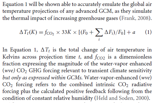



It is of the common kind, in effect a first order de

d( ΔT)/dt = a F

where F is a combination of forcings. It is said to emulate well the GCM solutions; in fact Pat Frank picks up a fallacy common at WUWT that if a GCM solution (for just one of its many variables) turns out to be able to be simply described, then the GCM must be trivial. This is of course nonsense - the task of the GCM is to reproduce reality in some way. If some aspect of reality has a pattern that makes it predictable, that doesn't diminish the GCM.

The point is, though, that while the simple equation may, properly tuned, follow the GCM, it does not have alternative trajectories, and more importantly does not obey physical conservation laws. So it can indeed go off on a random walk. There is no correspondence between the error propagation of Eq 1 (random walk) and the GCMs (shift between solution trajectories of solutions of the Navier-Stokes equations, conserving mass momentum and energy).

On Earth models

I'll repeat something here from the last post; Pat Frank has a common misconception about the function of GCM's. He says that
"Scientific models are held to the standard of mortal tests and successful predictions outside any calibration bound. The represented systems so derived and tested must evolve congruently with the real-world system if successful predictions are to be achieved."

That just isn't true. They are models of the Earth, but they don't evolve congruently with it (or with each other). They respond like the Earth does, including in both cases natural variation (weather) which won't match. As the IPCC says:
"In climate research and modelling, we should recognise that we are dealing with a coupled non-linear chaotic system, and therefore that the long-term prediction of future climate states is not possible. The most we can expect to achieve is the prediction of the probability distribution of the system’s future possible states by the generation of ensembles of model solutions. This reduces climate change to the discernment of significant differences in the statistics of such ensembles"

If the weather doesn't match, the fluctuations of cloud cover will make no significant difference on the climate scale. A drift on that time scale might, and would then be counted as a forcing, or feedback, depending on cause.

Conclusion

Error propagation in differential equations follows the solution trajectories of the differential equations, and can't be predicted without it. With GCMs those trajectories are constrained by the requirements of conservation of mass, momentum and energy, enforced at each timestep. Any process which claims to emulate that must emulate the conservation requirements. Pat Frank's simple model does not.