The GISS V4 land/ocean temperature anomaly was 1.26°C in February 20120 up from 1.10°C in January. That compares with a 0.053deg;C rise first reported in the TempLS V4 mesh index (now 0.073°C with later data). It was the second warmest February in the GISS record, just 0.11°C behind than the El Niño 2016, for which February was the peak.
As usual here, I will compare the GISS and earlier TempLS plots below the jump.
Friday, March 13, 2020

Friday, March 6, 2020
USA Temperatures; comparison of Moyhu results with NOAA.
This is a continuation of my earlier post on ConUS temperatures. I'll compare the time series results with those of the NOAA datasets ClimDiv and USCRN. My series are labelled GHCN_a, for the calculation using GHCNM V4 adjusted, GHCN_u for unadjusted, and MoyCRN for my calculation using CRN data. The data is as in the previous post. I'll start with the period 2005-2019, since this is where there is USCRN data. I'll use that period for the anomaly base throughout. Here is a graph of the various time series:
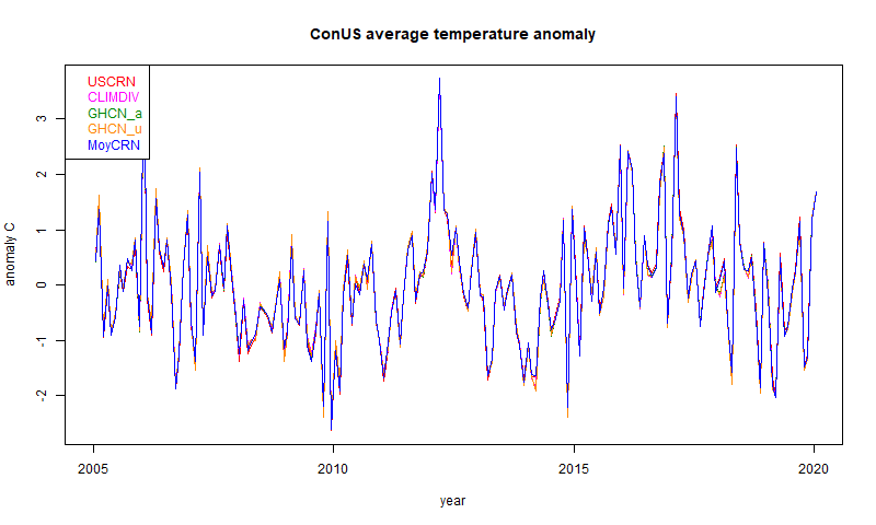
They are so close that the differences are hard to see. It is easier with a 12-month running mean, mainly because the y-axis doesn't have to cover such a large range: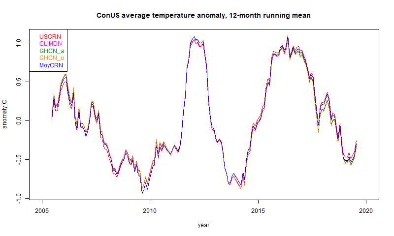
You can see that they are still very close, with some small difference between CRN and the other data. I can quantify this with a table of standard deviation of differences (unsmoothed data):
The very close results are between GHCN adjusted and unadjusted. Here the stations and the methods are the same, so the only difference is the adjustment of the data. And it is very small. The difference between the GHCNs and NOAA's ClimDiv is larger, but still very small.
The two CRNs show a larger difference again, but the largest is between the CRN groups and the others. As I said in the last post, I don't think this reflects different accuracy of the stations; CRN are presumably better. It reflects the dominance of location uncertainty in the spatial averages. That is, how much spread would you see if you measured at different places. Or, how well do you real think the infilling represents the unmeasured regions. Of course, the different coverage gives a check; I showed in the last post a difference plot in one month between the sparse CRN and the dense ClimDiv.
I have also shown the trends, in °C/century. These are very uncertain on such a short period, and you might be surprised at their size, since the plot doesn't reflect that by eye. But a trend of 2 °C/Cen rises only 0.3°C in this period. The closeness reflects that shown in the sd table. I don't think much should be made of the fact that CRN shows a higher trend.
Over a longer period, the CRN results do not cover, and the other data diverge more. The different adjustment policies start to show. Here is the period since 1900. I'm now using a 5 year running mean to make the differences clearer:

Now there is an obvious difference between the adjusted and unadjusted. My GHCN_a still agrees quite well with ClimDiv. Again the differences can be quantified in the reduced table of standard deviations:
The trends (in °C/Cen) again tell the story. Adjustment makes a big difference, as was noted back in USHCN V1. USHCN did both homogenisation and explicit TOBS adjustment, and I believe ClimDiv, which replaced it, does the same. GHCN relies on the pairwise homogenisation to cover the TOBS effect, and on this accounting it seems to do that very well.
Of course, some would say that this means that more than half the (modest) ConUS warming is created by adjustments. The proper scientific view is that unadjusted readings had a spurious cooling bias, which should be corrected. The sources of this are real and known:
They are so close that the differences are hard to see. It is easier with a 12-month running mean, mainly because the y-axis doesn't have to cover such a large range:
You can see that they are still very close, with some small difference between CRN and the other data. I can quantify this with a table of standard deviation of differences (unsmoothed data):
| 2005-2019 | USCRN | CLIMDIV | GHCN_a | GHCN_u | MoyCRN |
| USCRN | 0 | 0.091 | 0.098 | 0.103 | 0.058 |
| CLIMDIV | 0.091 | 0 | 0.027 | 0.029 | 0.092 |
| GHCN_a | 0.098 | 0.027 | 0 | 0.01 | 0.096 |
| GHCN_u | 0.103 | 0.029 | 0.01 | 0 | 0.099 |
| MoyCRN | 0.058 | 0.092 | 0.096 | 0.099 | 0 |
| Trend | 3.103 | 1.957 | 1.958 | 1.76 | 2.616 |
The very close results are between GHCN adjusted and unadjusted. Here the stations and the methods are the same, so the only difference is the adjustment of the data. And it is very small. The difference between the GHCNs and NOAA's ClimDiv is larger, but still very small.
The two CRNs show a larger difference again, but the largest is between the CRN groups and the others. As I said in the last post, I don't think this reflects different accuracy of the stations; CRN are presumably better. It reflects the dominance of location uncertainty in the spatial averages. That is, how much spread would you see if you measured at different places. Or, how well do you real think the infilling represents the unmeasured regions. Of course, the different coverage gives a check; I showed in the last post a difference plot in one month between the sparse CRN and the dense ClimDiv.
I have also shown the trends, in °C/century. These are very uncertain on such a short period, and you might be surprised at their size, since the plot doesn't reflect that by eye. But a trend of 2 °C/Cen rises only 0.3°C in this period. The closeness reflects that shown in the sd table. I don't think much should be made of the fact that CRN shows a higher trend.
Over a longer period, the CRN results do not cover, and the other data diverge more. The different adjustment policies start to show. Here is the period since 1900. I'm now using a 5 year running mean to make the differences clearer:
Now there is an obvious difference between the adjusted and unadjusted. My GHCN_a still agrees quite well with ClimDiv. Again the differences can be quantified in the reduced table of standard deviations:
| 1900-2019 | CLIMDIV | GHCN_a | GHCN_u |
| CLIMDIV | 0 | 0.064 | 0.257 |
| GHCN_a | 0.064 | 0 | 0.23 |
| GHCN_u | 0.257 | 0.23 | 0 |
| Trend | 0.84 | 0.828 | 0.371 |
The trends (in °C/Cen) again tell the story. Adjustment makes a big difference, as was noted back in USHCN V1. USHCN did both homogenisation and explicit TOBS adjustment, and I believe ClimDiv, which replaced it, does the same. GHCN relies on the pairwise homogenisation to cover the TOBS effect, and on this accounting it seems to do that very well.
Of course, some would say that this means that more than half the (modest) ConUS warming is created by adjustments. The proper scientific view is that unadjusted readings had a spurious cooling bias, which should be corrected. The sources of this are real and known:
- TOBS - it makes a substantial difference whether daily reading of a a min-max thermometer is done in the afternoon, where it tends to double-count warm days, or in the morning, where it double counts cool minima. The times of reading are known, and the pettern is a shift toward morning reading. This is a quantifiable cooling bias, and must be adjusted for. It isn't optional.
- Measurement changes - firstly improved screening, and then MMTS, both produced lower readings. These can be identified as abrupt changes relative to neighbours, and again must be corrected.
Next steps
I plan to set this analysis up as a regular calculation, as with TempLS global, and post the results on the data page. I have now done a similar analysis for Australia, which I'll also write about. I'll also work on a page of maps of past months, and possibly seasons and years.Thursday, March 5, 2020
February in ConUS - surface anomalies mostly warm - new graphics.
This post follows one here where I described a new way of calculating an average temperature for a region like ConUS (USA, lower 48 states) and showed comparative graphics for January 2020. I use GHCN V4 data, and there is now enough out to do a February post. It was warm like January, in most parts. I'll link below to a set of numerical data for ConUS for all months since 1900.
I use 2005-2019 as the base period for anomalies, to make possible comparison with USCRN. But I won't show USCRN here, because the greater station numbers in GHCN give a better result. Probably in production I'll revert to the WMO base of 1981-2010. I use GHCN unadjusted here; visually, it makes no difference. Here is the result for February 2020:

I realised that I could also usefully compare this graphic with the WebGL global plots that I show as the data comes in. These are the most detailed early depictions of the data. Here is a zoomed extract from that source:

Both plots have the property that the color at each station is correct at that point, and elsewhere is interpolated. The WebGL plot is based on triangular mesh with linear interpolation; the new plot uses the Laplace infilling, which is smoother.
Next I'll show the corresponding plots for 2019. At some stage I'll set up a page which goes back further. This one is done in the usual style where the buttons below let you cycle through the months.
Historical results and comparisons.
I'll post soon with an analysis of comparison with other data. I'll post a link to the table here. The table shows the NOAA data for ClimDiv and USCRN, and my corresponding averages using data from GHCN V4 adjusted, unadjusted and USCRN. All results have been set to anomaly base 2005-2018.
Wednesday, March 4, 2020
February global surface TempLS up 0.053°C from January.
The TempLS mesh anomaly (1961-90 base) was 1.032deg;C in February vs 0.979°C in January. This was a contrast to the NCEP/NCAR reanalysis base index, which barely changed. It makes it the second warmest February in the record, just behind the El Niño 2016 at 1.133°C. That is remarkable, because in this index February was the warmest month of that very stong El Niño.
The prominent feature, as with January, was a huge band of warmth stretching from Europe through to E Siberia and China. Again N America was also warm, except for Alaska (cold). Greenland and the Arctic archipelago were also cool. Africa and S America were mostly warm, Antarctica mixed.
Here is the temperature map, using the LOESS-based map of anomalies.
 As always, the 3D globe map gives better detail.
The prominent feature, as with January, was a huge band of warmth stretching from Europe through to E Siberia and China. Again N America was also warm, except for Alaska (cold). Greenland and the Arctic archipelago were also cool. Africa and S America were mostly warm, Antarctica mixed.
Here is the temperature map, using the LOESS-based map of anomalies.
As always, the 3D globe map gives better detail.Tuesday, March 3, 2020
NCEP/NCAR reanalysis monthly surface temperature unchanged in February 2020.
The Moyhu NCEP/NCAR index came in at 0.554°C in February, following 0.552°C in January, on a 1994-2013 anomaly base. With December even warmer, that is a sustained period of warmth.
As with January, the main feature was a band of warmth from Europe right across Russia and Siberia. Again there was a complementary cold band across Arctic North America and Greenland. Elsewhere mixed, with cool seas around S America, and a cool region in the Sahara.
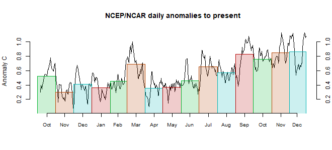
As with January, the main feature was a band of warmth from Europe right across Russia and Siberia. Again there was a complementary cold band across Arctic North America and Greenland. Elsewhere mixed, with cool seas around S America, and a cool region in the Sahara.
Thursday, February 27, 2020
USA Temperatures; averaging and graphics methods.
I have for many years been experimenting with methods for calculating average surface temperature anomalies from collections of station readings (including sea surface from grid, regarded as stations). I describe the history here. In the early days, I tried to calculate the averages for various countries and continents. With the coarse grids I was using at the time, and later meshes, I found the results unsatisfactory, and of limited scientific importance.
So I put more effort into developing global methods. There is a rather mathematical survey of these here. Briefly, there are six main types:
- The conventional grid analysis, averaging the measurements within each cell, and then getting an area-weighted average of the cells. I think this is very unsatisfactory since either the grid is very coarse, or there are cells with no data.
- Triangular mesh, with the sites as nodes. This has been my mainstay. But it is not very good at following national boundaries.
- A method where spherical harmonics are fitted and then integrated. This is now implemented as a general method for improving otherwise weak methods. The structure is instructive, but again, intrinsically global.
- A LOESS method, described here This has the characteristic of gathering information from as wide a net as needed; useful when stations get sparse, but not a respecter of boundaries.
- Most recently, a method using FEM shape functions. I think this may be best, in terms of getting the best representation on a relatively coarse grid. Again, not so good for boundaries, but it has as a special case, one of my earlier methods:
- Grid with infill (eg an early version here). The weakness of conventional gridding is that it does not use local information to estimate missing cells, and so the grid must be kept fairly coarse. But I have worked out a way of doing that systematically, which then allows much finer gridding. And that does have the incidental benefit of tracking national and land boundaries. It also allows a good graphics scheme. I'll say more about it in the next section. In this text, I'm using blue colors for the more technical text.
Infilling and diffusion - the Laplace equation.
The logical expression of using neighbour information is that empty cells should be assigned the average temperature of their neighbours. For an isolated cell, or maybe a few, you can do this directly. But with clumps of empty cells, some may have no known neighbours at all. But you can still maintain the requirement; a solution procedure is needed to make it happen.
The idealization of this is the Laplace differential equation, solved with Dirichlet boundary conditions expressing the known cells, and zero gradient (Neumann) conditions at the boundaries (not needed for the globe). That equation would describe a physical realisation in which a sheet of metal was kept insulated but held at the appropriate temperatures in specified locations. The temperatures in between would, at equilibrium, vary continuously according to the Laplace equation.
This is a very basic physical problem, and methods are well established for solving. You just write a huge set of linear equations linking the variables - basically, one for each cell saying that it should be the average of the neighbours. I used to solve that system just by letting it play out as a diffusion, but faster is to use conjugate gradients.
Once the data-free cells are filled, the whole grid can be integrated by taking the area-weighted average of the cell values.
In one dimension, requiring each unknown value to be the average of its neighbours would lead to linear interpolation. Solving the Laplace equation is thus the 2D analogue of linear interpolation.
Graphics and gridding the region
I mentioned the usefulness for graphics. I just draw a point of the appropriate color for each cell. For ConUS (contiguous) I typically use grid cells of about 20km edge, giving about 20000 for the country, and so quite good resolution. I will give examples shortly.As far as getting a grid of the US, say, one might look on public data for a lat/lon land mask. There is a lot of choice for physical land, but I found it harder for ational boundaries. But anyway, there is another consideration; projection. A lat/lon grid is not isotropic. N-S neighbours are further away than E-W. Proper use of the Laplace equation would require allowance for this. And anyway, good graphics would require an equal area projection.
So I decided to make a map, after projection, using the R maps package. I can extract a specification of the US as a complex polygon. I remap the data, first onto a sphere, then project that on to a plane tangent to the sphere at the US center (I used 37N, 97W). Then I output that on a suitable small scale as a BMP file (uncompressed), and read off the pixels. That gives a regular grid, not lat/lon, which is very close to isotropic - cells are close to square (see notes below).
The task of mapping requires another solution of the Laplace equation, applied to the cell averages of the station anomalies.
Data sources
I was interested to see the result for ConUS because GHCN V4 monthly has a dense network of nearly 12000 US stations. I used both the unadjusted and adjusted versions. There is also the data from USCRN. Here I use just the 115 commissioned stations, for which some were reporting in 2002, but I use only since 2005, when there were enough to try for a regional average. These stations are evenly distributed, and of high quality, with almost no missing (monthly) data recently. But they are sparse.NOAA posts monthly averages ClimDiv and USCRN which I can use for comparison. I'll do that in detail in my next post. GISS posts unfortunately only annual averages, but I can use that for a check. I'll talk more about NOAA's graphics below. They feature the anomaly graph in their national climate reports, although they describe them as "Average Temperature Departures" from an absolute spatial average, so it may not be the same thing.
An example - USCRN
For the graphics I solve the Laplace equation on a finer mesh of about 10x10 km. The plot of the solution for USCRN shows the good and bad features of the Laplace interpolation method:
The stations are shown with small dots. With this, and the next plot, you can remove the stations and the state borders with the checkboxes top right. Mostly the interpolation is smooth, with a few that stand out creating a small dimple. The color actually at the station is in this image exact. There are just 115 stations, so that is a fairly good result. The anomaly base is 2005-2019, which is what is available with USCRN, and so I use the same base when comparing with GHCN.
Now here is a plot of the same month, with the much more numerous GHCN V4 data (5263 stations reporting)
Obviously there is much more detail, not resolved by the CRN infill. The integral is almost identical (1.694 vs 1.689). I'm using unadjusted GHCN data here, although it makes very little difference. I think the results show very good spatial concordance between the GHCN stations, and that the patterns that they reveal are signiicant.
Comparison with NOAA
I mentioned that NOAA publishes anomaly maps in the monthly National Climate Reports (January 2020). Here is their plot:
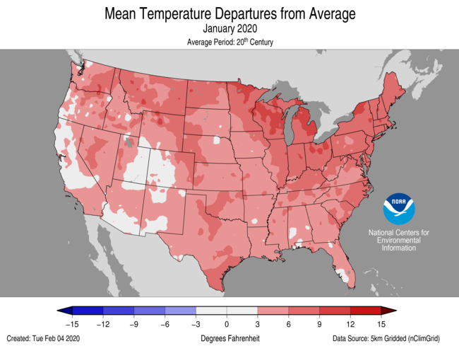
Here is my plot, now using the colors (almost) and levels of the NOAA plot. I also use the same anomaly base (20th century) and now use adjusted GHCN, although again, it makes very little difference over recent times. Temperatures now in Fahrenheit.
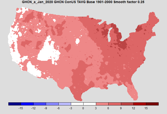
It's pretty similar. Mine is a little cooler on the west coast. The agreement is not because of identical data, as the ClimDiv set used by NOAA is somewhat more extensive.
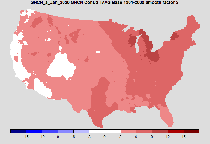
I've shown a smoothing factor; 0.25 is essentially no smoothing. Here is a plot which smooths out some of the speckles without changing the result substantially
Next steps
I'll post very soon a much more detailed comparison of time series. Generally, my GHCN based averages agree very well with the NOAA Climdiv series since 2005; the agreement with the CRN average, both my GHCN and Climdiv, is not as close. In earlier times, the effects of differing adjustment do start to show through. I think the inferior agreement of the CRN average emphasises that the main error in regional temperature averaging is not station imperfections, but coverage uncertainty. The finer grade GHCN shows how a different location of the CRN sites, no matter how good they are, would give a different result.
I started looking at the US results because they are often misused by sceptics, and I wanted a good independent method of checking on the sometimes opaque NOAA procedures.
I'll probably add monthly updates to the latest data page. I'll do something similar with Australia.
Some technical notes on implementation.
1. It took a while to get the Laplace operator right. I do the following steps:
- Make an nx4 matrix of the neighboring values for the n stations. Calculate the row sums (not means).
- Make a diagonal consisting of the number of items in each row. Add B ( a large number, say 100) to the cells with data.
- Make another vector with B's on the cells with data, 0 elsewhere.
- The symmetric part of the implementation is done by multiplying the coefficients from 2 by the values, and subtract the rowsums from row 1.
- This is then scaled by the inverse of the diagonal, and right multiplied by the vector from 3. These operations can be deferred; the conjugate gradient iteration, which requires symmetry, should be done on the symmetric part and the scaling later.
I needed a scheme to deal with the imperfect coast alignment (and possibly inaccurate lat/lon in the GHCN inventory). Some stations are out to sea. I linked them with the nearest (usually adjacent) cell in the US grid. The Channel Islands of California resisted this process, and I had to omit them.
I use a TempLS-like convergence to get the station normals (offsets). They are not necessarily the same as those used in the global calculation. It is an independent analysis. It takes only a minute or so for the GHCN case (CG iterations are about 30-100 per month); CRN is longer, because there is more infilling to do. Those numbers are for the 20 km cells; 0 km are much slower.
Islands without data can be a problem, since they make the solution indeterminate, which slows the iterative solution. I added a very small number (1e-6) to the diagonal, which fixes the island solution at zero (anomaly). Fortunately this was a rare problem.
I described above the way I projected the US onto the plane. I rotated the spherical coords so that the centre (37N 97W), was at (0N, 0E), which is the (0,0,-1) 3D point. Then I projected onto the z=-1 plane from the point (0,0,2). This minimises the distortion near the centre, which is to say, for most of the USA.
Update: In comments, MMM suggested a difference plot between CRN and GHCN would be interesting. I agree. Although the differences are not large, they do not seem to be random. Here is the plot:
Saturday, February 15, 2020
GISS January global up by 0.08°C from December.
The GISS V4 land/ocean temperature anomaly was 1.18°C in January 2019, up from 1.10°C in December. That compares with a 0.047deg;C rise first reported in the TempLS V4 mesh index (now 0.079°C with later data). It was the warmest January in the GISS record, just 0.01°C warmer than the El Niño 2016.
As usual here, I will compare the GISS and earlier TempLS plots below the jump.
As usual here, I will compare the GISS and earlier TempLS plots below the jump.
Subscribe to:
Posts (Atom)


 Posts

