Climate and the Lorenz attractor, 3D interactive model.

In my previous post, I described some recent blog discussion of chaos and climate models (GCMs), and gave my views on the relation to Navier-Stokes solution and CFD. People who write about chaos tend to focus on the trajectories, and their touchy relations to starting point, claiming this undermines GCMs. They should instead focus on the attractors, which are independent of start point sensitivity, and are the analogue of climate. And I contend that attractors have a manageable relation (see Appendix for math) to parameters that may vary - forcings for climate, or coefficients in a chaos differential equation.

In this post, I'll focus on the Lorenz DE's



These have, for various parameters values, chaotic solutions with interesting trajectory paths often shown:

A trajectory for the standard Lorenz parameters σ=10, β=8/3, ρ=28. Often displayed without mentioning that specific parameters are required.	An attractor (due to Anders Sandberg, Oxford) parameters not specified but seems close to standard.

This post provides below a Javascript interactive display of the Lorenz system. You can choose parameters and start points. It is built on the WebGL of my standard Earth view, so you can rotate with mouse as if it were in a trackball, and also magnify or reduce by right button dragged vertically. There is also provision for viewing separate trajectories, and for running an animation of their evolution.

The general idea is that you can compare the effect of changing start points, with comparison red/blue trajectories, and also see the very great range of different attractors that result when the parameters are changed, However, the changes are continuous. What I'd like to get to eventually (future post) is a possible relation between an average of trajectories and the attractor. That would help understand how GCM runs can be averaged to get a climate evolution.

Chaos, CFD and GCMs.

There has been a flurry of skeptic blogging (and commentary from me) on chaos and climate models. It's generally along the lines that chaos renders GCMs unworkable because of small changes magnifying or some such, with words like coupled and non-linear. Kip Hansen has a series at WUWT, finishing here. Like many such, it shows the Lorenz trajectories produced by a set of three slightly non-linear equations. I'll develop that with a gadget to explore these curves and their attractor in a future post. Tomas Milanovic has one of an intermittent series of posts (latest "Determinism and predictability") at Climate Etc, of which the general theme is the unsolvability of Navier-Stokes equations due to some effect of non-linearity negating proof of existence and uniqueness, or some such.

My standard response to all this is, look at Computational Fluid Dynamics (CFD, which has been my professional activity for the last thirty years). It is a major established engineering tool based on numerically solving the Navier Stokes equations, and has dealt with the chaos (turbulence) from the beginning. And the climate models are just large scale CFD. There are certainly difficulties with the solution, mainly to do with the necessary sub-grid modelling (in both CFD and GCMs). But they aren't to do with the fact that the solutions don't relate to initial conditions. In fact, that is a benefit, since initial conditions are hardly ever known accurately.

And the theoretical issues of existence and uniqueness etc don't impinge on practice. Algorithms are used which generate solutions on a gridded or meshed space with time stepping. These solutions satisfy on that scale the conservation laws of momentum, mass and energy, which are also expressed by the N-S equations. If you find such a solution, it doesn't matter whether it's existence could be proved in advance. As for uniqueness, the solution procedure itself will generally indicate whether different solution pathways are possible. One CFD scientist, David Young, has been objecting that some recent work, in which he has a part, does show non-unique solutions. But as far as I see, this is in situations like near-stall on a wing, where reality itself is far from predictable.

The CE post had an odd answer to this - yes, CFD works, but only on a scale of up to a few metres. This is of course unphysical - there is no such restriction on the physical laws, nor in the discretised algorithms is any physical scale limitation built in. And of course, GCM's are just Numerical Weather Prediction (NWP) programs, run for longer periods. Most sensible people concede that these work quite well, despite the many km scale.

What people who like to show fancy chaos pictures rarely dwell on is the nature of attractors. These are what distinguish chaos from randomness. And they are typically the results that are sought from CFD analysis. In CFD, initial conditions are usually just a nuisance (because you rarly have good data, and when you try and specify them, there is usually something that will generate unintended disturbances). The standard remedy is to run the program for a while to let these settle out. This takes advantage of the fact that initial conditions are swept away in chaos. GCM's do the same. They typically "wind back" to start at some time well before the period of interest. This would be bad if initial conditions mattered, because data back then is less reliable. But it isn't bad, because they don't. Again, it is better to let artefacts settle before the solutions are needed.

This lack of concern with initial conditions in a search for attractors, relates to the frequent criticism of GCMs as predictors. GCM's find out about climate (attractor), but don't predict the trajectories that converge to them (weather). That relates to the initial condition issue - models can only generate trajectories that are possible in the circumstances, not ones that will reproducibly happen.

When trying to explain why GCMs do really work, and attractors are the key, I often post this GFDL video of modelled ocean SST over seasons. I say that it shows many transient effect, from various eddies to longer term events like ENSO. None of these are predictions for Earth. The actual eddies won't happen, nor will the ENSO events, at least not at the stated times. But this solution which just came from specifying bottom topography and various long term forcings (energy input) comes up with familiar patterns like Gulf Stream and other major ocean currents. The wiggles vary, but the current is there. There is underlying physics which determines the transfer of heat from the Caribbean to the North Atlantic. And GCMs can tell you how that effect of physics will relate to changes in forcing. Anyway, here is the video:



In my next post, I'll develop the notion of an attractor using the simple Lorenz system of differential equations. These show two important things. Trajectories follow a path with a pattern that is, after some convergence from the initial point, similar for all cases. This is the attractor, and in contrast to the hypersensitive dependence on initial conditions, the dependence of that trajectory on the three parameters of the system is gradual, although over the full range allows many very different shapes. To do this, I'll show a Javascript/WebGL gadget that allows you to vary initial conditions and parameters, and visualise the trajectories in 3D.

GISS down 0.06°C in September

GISS is down from 0.97°C in August to 0.91°C in September. This compares with a larger fall of 0.12° in TempLS mesh, and contrasts with the small rise in the NCEP/NCAR index. It is still the warmest September in the record (just ahead of 0.90°C in 2014). It really hasn't cooled since May, and a record hot 2016 is ever more likely.

As I mentioned in the TempLS post, the dominant effect on recent changes is Antarctica. TempLS rose strongly in Aug, and dropped in Sep; GISS responded in the same way, but to about half the extent. I expect NOAA and HADCRUT to be less affected again.

I'll show the map comparisons below the fold. The updated comparison plots with 1998 are here

TempLS Surface temperature down 0.12°C in September

The Moyhu TempLS mesh index fell in September to 0.736°C, down from from 0.855°C in August. That still makes it the hottest September in the record. TempLS grid fell 0.04°C fro 0.785°C to 0.744°C. The recent ups and downs mainly relate to Antarctica, which was very cold in July, very warm (relatively) in August, and about normal (on average) in September. TempLS mesh followed this closely, while TempLS grid regards a lot of Antarctica as missing values, and so downweights the changes. This is reflected in the other indices - GISS and BEST rose like TempLS mesh, while NOAA (0.05°C) and HADCRUT changed mush less. I would expect GISS to also drop this month, but NOAA and HADCRUT maybe not.

In terms of regions, there isn't much unusual outside Antarctica. Siberia, Europe, E US and Alaska fairly warm, with just Australia on the cold side. I can vouch for that, though we were on the fringe of the cold region shown. With other indices, UAH lower trop was steady, while RSS rose by about 0.1. All seem set for a record warm 2016.

On housekeeping, Google says they are looking into the blogroll issues - still out.

The map is below the jump; report at the data page here.

Reanalysis index up 0.047°C in September

The Moyhu NCEP/NCAR index rose in September to 0.475°C, up from 0.428 in August. This brings it back to about the level of May. There was then a drop to June, followed by a gradual increase to now. This seems to be associated with ENSO-neutral conditions. And as usual recently, it was the hottest month of its kind in the record. Next month will test this trend of records, since Oct 2015 was very warm.

On other matters, I apologise for the absence of blogroll, search etc. Apparently Google Blogger has recalled them for repair. I'm told they should reappear soon.

Twelve coin problem

Update: New constructive algorithm appended.

Things are a bit quiet in climate blogging - so with a weekend coming I'll honor my ancient promise of diverting to some recreational math. I saw a few weeks ago a mention at Lucia's of the old twelve coin problem. Twelve coins, one of which is fake and of different weight to the others, and to be found with three weighings on a balance (Update: the usual spec, as here, is that you also have to say whether it is heavier or lighter). This first came to prominence in WWII, when it was said to have become a distraction to the war effort in places like Bletchley Park, leading to suspicions that it had been planted by the Germans. A suggested counter was for the RAF to drop it on Germany.

I first encountered it when I started University; it was posed in circumstances where I was expected to be able to solve it, and I was embarrassed. A year later, I went to a lecture on information theory (newish in those days). I was struck by the proposition, helpful in later years, that the information in a result was a function of prior uncertainty. So that is the clue - each weighing should be arranged so each of 3 outcomes was as near equally probable as could be managed, maximising prior uncertainty. Then I could solve it easily, and also versions with more coins.

The basic constraint is that in N weighings there are 3^N possible outcomes, while with n coins, there are 2n situations to resolve, since only once coin is false, and could be heavy or light. So for 12 coins, there are 24 possibilities and 27 outcomes of 3 weighings, so it is tight but possible. An alternative to the equiprobable outcome method is a requirement that each weighing should be so that each outcome was resolvable with the remaining weighings.

When I saw it mentioned again, I started thinking of a constructive algorithm that would also prove feasibility for all cases where there were enough results to theoretically resolve. I had an idea of describing the proof, but then my other recent hobby of Javascript programming seemed it might help. So I've made an interactive version (below) with the information needed to solve.

You can choose a number of coins up to 121, and then start (or restart any time). There are boxes for left, right and off-scale. The buttons representing coins have colored bands top and maybe bottom. The top band is what I call the HL score. Initially each coin might the bad one, heavy or light (HL). But once there has been a weighing that tilted, some possibilities fail. On the side that dropped, the coins could no longer be light, hence H. On the other side, they are L. And any not on the balance must be good (G). So the total number of possibilities remaining is the HU score = 2*HL+H+L.

There is another more subtle score - DU. This applies to the coins on the balance before weighing, and relate to whether you will gain information if the left balance goes down or up. HL coins will always become either H or L, so they are not scored. But if left pan down, then L on left or H on right would then be known to be good, so they are marked as D; if the left pan went up, that would tell nothing new about D coins. And similarly H on left or L on R would be counted as R.

You can move coins to the right (cyclic) by mouse click, or left by click with shift key pressed. If they are H or L, you will see the lower DU bar change as they move. When a weighing has been set up, click the weigh button.

The color scheme for top bars is HL black; H orange; L blue and G yellow. For the bottom, only H and L coins on the balance have color, and it's red for D, green for U. Here is an image of the gadget immediately following afirst weighing of 12 coins. Note the balance tilt. The four coins on the left are now H because they are on the heavy side, and U because they are H and left. On the right, they are L similarly, and also U. The off balance coins are all G, yellow.



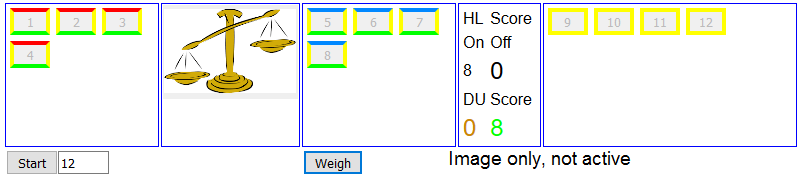
You'll see a table with the HL counts for on and off, and the D and U counts. Three are in large fonts, and those are the ones needed for solution. The strategy is that for every weighing, the D and U should be as near equal as possible, and the off HL score should be about half the on. More critically, each should be ≤ 3^M, where M is the number of weighings to follow after the one being set up. So in the image, for the next weighing, these numbers should all be ≤3. So take 3 off, then swap the others until the D and U scores are each ≤3. You'll see that as you rearrange, the system pads with known good coins (if available) to retain balance, and removes surplus. You can try to minimise usage of dummies; you should be able to reduce the need to at most two. If known good coins aren't available (first weighing), don't worry; the system will imagine them present.

So here is the gadget. Just press start, then move coins for weighing with click and shift-click, bearing in mind the above strategy. As long as the three big numbers are ≤ 3^M, you can solve in minimum weighings. It is solved when there is just one coin with H or L color showing.

I have to say, it is now a bit mechanical. You don't need to know the coin numbers, or even what the colors mean, as long as you keep your eye on the scores. But the Javascript isn't solving it - it's just adding up what you could count yourself, but displayed in a helpful way.

Update I have changed the DU score to count 1 each for HL (black) coins. This is more consistent when there are such coins. It means that all 3 large font numbers should now be made as nearly as possible equal an ≤3^M.

Update - proof

I originally planned this post as a constructive proof - show a method that is sure to work. I think the scoring goes a long way there. But a method can be spelt out. Suppose we have a set of coins with HL score g≤3^N+1, to resolve in N+1 weighings. It's enough to show that a weighing can be made to reduce this to an assured score h≤3^N. And the point of the big font numbers in the gadget is that they are the respective HL scores after each possible outcome.

Let g=2*p+q, where 3^N≥p≥q≥0. Normally p=3^N is OK, but if that leaves q<0, you can reduce p until q is positive. Then take a set of coins, HL score q (including all known good ones), to be kept off the balance. If all coins have HL score 2 (as at the start), that's still possible, because g and hence q must be even.

Then put the remaining coins one by one on the balance. Depending on what side, the D and U scores will increment by 1 or zero. Put all the H coins on first, alternating sides so the gap between D and U is never more than 1. Then the L, also so as to increase whichever of D,U is less. That will also alternate, so there will be a max imbalance of coin numbers of 2. Then finally, if there are HL coins, put them on whatever side improves coin number balance; each will increase both D and U by 1.

This ensures D+1≥U≥D. And since D+L is the HU score, when loaded, D=U=p≤3^N. Since D,L and q are the respective HL scores after each possible balance result, and each ≤3^N, that completes the proof.

Numbers of coins on each pan may differ by up to two. After the first weighing, this can be balanced by adding known good coins. On the first weighing, if g<3^N-1, you can always choose p even, so the coins can split equally. In the worst case where g=3^N-1 (eg 13 coins in 3 weighings) an external known good coin is needed.

Update: New constructive algorithm.

I thought of a simple constructive algorithm, with notation. Whenever a coin is on a tipped balance, you have half-knowledge about it. If it is on the down side, you know it can't be light, so I call it a H coin. On the other side, L. A known good coin I'll call G; one not half-known U

I'll call an odd trio, one that is HHL or HLL. An odd trio is the most that can be resolved in one weighing. You weigh an HL against a GG. If HL tips up, L is the culprit, if down, H. If balanced, you know the coin taken off is the bad one, and you know if it is H or L.

Any half-known duo duo can be resolved by just balancing one coin against a G. So at the end of the second weighing, we must have nothing harder than an odd trio.

So start with 8 on the scale, 4 off. This makes the 3 outcomes equally likely. If =, the 8 are G. Put 3 of the 4 on the scales, with one G. If = again, there is just one coin left, and can be weighted against a G. Otherwise, we have an odd trio.

If the first weighing tipped, remove a HHL, Leave a HLL in place, and interchange the remaining HL. Add a G to even coins for next weightng. If =, the odd trio HHL taken off has to be resolved. If it tips the HLL has it. If it tips the other way, the HL needs to be resolved.

In this table, each cell contains 3 groups. The first is the coins set aside, the other two are those placed on the scales. It stops after third weighing, because all outcomes can be resolved as odd trio or easier in third weighing.

Weighing 1	UUUU UUUU UUUU
Outcome 1	GGGG HHHH LLLL			UUUU GGGG GGGG
Weighing 2	HHL HGL LLH			U UU UG
Outcome 2	HHL GGG GGG	GGG HGG LLG	GGG GGL GGH	U GG GG		G HH LG
Weighing 3	H HL GG	L HL GG	L H G	G U G		H HL GG

CRUTEM (HADCRUT) versions are documented and accessible

I have encountered at WUWT ongoing complaints about HADCRUT 4 updates. It is currently in a thread here, but goes back to an earlier post here. The complaints typically say that the new versions always raise current anomalies, and suggest that they are poorly documented. In fact, the changes are extensively noted; see directory here.

In the earlier thread Tim Osborn commented here, to say mainly that the changes were due to changes (mainly additions) to station data, and listed the particular additions to HADCRUT 4.3. He also later made the important point that there is a good reason why the trends rise with new data. HADCRUT is a land/ocean set, but the empty cells are mainly on land, and the new data allows some of them to be filled. HADCRUT is an average by grid (area-weighted), in which cells without data are simply not included. That has the effect of assigning to them the global average, which is dominated by sea temp. If new stations assign to empty cells genuine land values, that will increase the trend, because land is warming more rapidly. HADCRUT had artificially low trends because of this missing value policy, as was remedied by Cowtan and Way (2013) - discussed here in a series of posts, with links here.

But another feature of HADCRUT transparency is insufficiently appreciated. For Ver 4, at least, they give a complete listing of station data for each version, with each station file documented. Here is a typical version file; it is for 4.4, but just change that URL to 4.2 or whatever you want. Each links to a zip file of the station data for that version (except for Poland), which has a URL like http://www.metoffice.gov.uk/hadobs/crutem4/data/previous_versions/4.4.0.0/station_files/CRUTEM.4.4.0.0.station_files.zip. I'm spelling out the URL because if you click on it, it will immediately download about 18Mb. But again, you can edit for other versions.

I couldn't find, though, inventory files, except for 4.5. But it's easy enough to make them from the file headers. So I've done that, and placed the zipfile here (612 Kb). It has a csv file for each of 4.2-4.5, and the columns have 3 letter abbreviations meaning:

• num - a unique HAD station number
• nam - name of station
• cou - country name
• lat - latitude in deg
• lon - longitude in deg
• alt - altitude in m
• sta - start year of data
• end - end year
• sou - source id code

UEA has an explanations file here, which is the best source I have found for the source id codes, but unfortunately it dates from 2012, and there is a new one pretty much with each new dataset that has come in. I'd be glad to hear of something more recent. It isn't really a problem, because the later numbers are in order of addition, so are easy to work out. Note that the files are in number order, but countries are not necessarily consecutive blocks.

So I thought I would just post this information, so that people who really want to know what HADCRUT is up to can look it up. I may in future produce a Google map.