Anyway, for the record, I would like to set down some clarification of what the scenarios for the predictions actually were, and what to make of them. Some trouble has been caused by Hansen's descriptions, which were not always clear. This is exacerbated by readers who interpret in terms of modern much discussed knowledge of tonnage emissions of CO2. This is an outgrowth of the UNFCC in early 1990's getting governments to agree to collect data on that. Although there were estimates made before 1988, they were without benefit of this data collection, and Hansen did not use them at all. I don't know if he was aware of them, but he in any case preferred the much more reliable CO2 concentration figures.
Sources
I discussed the sources and their origins in a 2016 post here. For this, let me start with a list of sources:- Hansen's 1988 prediction paper and a 1989 paper with more details, particularly concerning CFCs
- Some discussions from 10 years ago: Real Climate and Steve McIntyre (later here). SM's post on scenario data here. See also Skeptical Science
- A 2006 paper by Hansen, which reviews the predictions
- From that 2007 RC post, a link to data files - scenarios and predicted temperature. The scenarios are from the above 1989 paper. I'll call this data Scen_1
- A RealClimate page on comparisons of past projections and outcomes
- A directory of a slightly different data set from Steve McIntyre here, described here. I'll call that Scen_2. The post has an associated set of graphs. It seems that SM calculated these from Hansen's description.
- A recent Real Climate post with graphs of scenarios and outcomes, and also forcings.
- I have collected numerical ascii data in a zipfile online here. H88_scenarios.csv etc are Scen_1; hansenscenario_A.dat etc are Scen_2, and scen_ABC_temp.data.txt is the actual projection.
Hansen's descriptive language
The actual arithmetic of the scenarios is clear, as I shall show below. It is confirmed by the numbers, which we have. But it is true that he speaks of things differently to what we would now. Steve McIntyre noted one aspect when Hansen speaks of emissions increasing by 1.5%:"One idiosyncrasy that you have to watch in Hansen's descriptions is that he typically talks about growth rates forthe increment , rather than growth rates expressed in terms of the quantity. Thus a 1.5% growth rate in the CO2 increment yields a much lower growth rate than a 1.5% growth rate (as an unwary reader might interpret)."
Hansen is consistent though. His conventions are
- Emissions of CO2 are always spoken of in terms of % increase. Presumably this is because he uses tonnages for CFCs, where production data is better than air measurements, and % works for both. Perhaps he anticipated having CO2 tonnages some time in the future.
- So emissions, except for CFCs, are actually quantified as annual increments in ppm. He does not make this link very explicitly, but there is nothing else it could be, and talk of a % increase in emissions translates directly into a % increase in annual ppm increment in the numbers.
- As SM said, you have to note that is is % of increment, not % of ppm. The latter would in any case make no sense. In Appendix B, the description is in terms of increments
- Another usage is forcings. This gets confusing, because he reports it as ΔT, where we would think of it in W m-2. He gives in Appendix B for CO2 as the increment from x0=315 ppm of a log polynomial function the current ppm value. This is not far from proportional to the difference in ppm from 315. Other gases are also given by such formulae.
- An exception to the use of concentrations is the case of CFCs. Here he does cite emissions in tons, relying on manufacturing data. Presumably that is more reliable than air measurement.
Arguments
Update. Eli notes in comments that he went through a lot of this in 2006, here, and continued here. I'll show his forcing graph below.
- Ignoring scenarios
Many people want to say that Hansen made a prediction, and ignore scenarios altogether. So naturally they go for the highest, scenario A, and say that he failed. An example Noted by SkS was Pat Michaels, testifying to Congress in 1998, in which he showed only Scenario A. Michaels, of course, was brought on again to review Hansen after 30 years, in WSJ. This misuse of scen A was later taken up by Michael Crichton in "State of Fear", in which he said that measured temperature rise was only a third of Hansen's prediction. That was of course based, though he doesn't say so, on scenario A, which wasn't the one being followed.
In arguing with someone rejecting scenarios at WUWT, I was told that an aircraft designer who used scenarios would be in big trouble. I said no. An aircraft designer will not give an absolute prediction of performance of the plane. He might say that with a load of 500 kg, the performance will be X, and with 1000 kg, it will be Y. Those are scenarios. If you want to test his performance specs, you have to match the load. It is no use saying - well, he thought 500 kg was the most likely load, or any such. You test the performance against the load that is actually there. And you test Hansen against the scenario that actually happened, not some construct of what you think ought to have happened. - Misrepresenting scenarios
This is a more subtle one, that I am trying to counter in this post.People want to declare that scenario A was followed (or exceeded) because tonnage emissions increased by more than the 1.5% mentioned in Hansen. There are variants. These are harder to counter because Hansen made mainly qualitative statements in his text, with the details in Appendix B, and not so clear even there.
But there isn't any room for doubt. We have the actual numbers he used (see sources). They make his description explicit. And they are defined in terms of gas concentrations only (except for CFCs). Issues about how tonnage emissions grew, or the role of China, or change in airborne fraction, are irrelevant. He worked on gas concentration scenarios, and as I shall show, the match with scenario B was almost exact (Scen A is close too).
Scenario arithmetic for CO2
. As mentioned, Hansen defined scenario A as emissions rising by 1.5% per year, compounded. The others differed by a slightly slower rate to year 2000. Scenario B reverted to constant increases after 2010, while scenario C had zero increases in CO2 ppm thereafter. See the graphs below. With all the special changes in Scenario B, it still didn't get far from Scenario A over the 30 years.The basic arithmetic for Scenario A is that, if a1, a2, a3 are successive annual averages of CO2 ppm, then
(a3-a2)/(a2-a1) = 1.015
or the linear recurrence relation a3 = a2 +1.015*(a2 - a1)
There is an explicit solution of this for scen_2, which is the set Steve Mc calculated:
CO2 ppm = 235 + 117.1552*1.015^n where n is the number of years after 1988. That generates the dataset.
The formula for the actual Hansen set is slightly different. Oddly, the increment ratio is now not 1.015, but 1.0151131. This obviously makes little difference in practice; I think it arises from setting the monthly increment to 0.125% and compounding monthly. However
1.00125^12 = 1.015104 which is close but not exact. Perhaps there was some rounding.
Anyway, with that factor, the revised formula for Scen_1 is
Scen A: CO2 ppm = 243.8100 + 106.1837*1.0151131^n
Scenario B is much more fiddly from 1988-2000, though a straight line thereafter. Hansen describes it thus
"In scenario B the growth of the annual increment of CO2 is reduced from 1.5% yr-1 today to 1% yr-1 in 1990, 0.5% yr-1 in 2000, and 0 in 2010; thus after 2010 the annual increment CO2 is constant, 1.9 ppmvyr-1".
It isn't much use me trying to write an explicit formula for that. All I can report is that Scen_1 does implement that. I also have to say that this definition is too fiddly; the difference between A and B after all that fussy stuff is only 0.44 ppm at year 2000.
Scenario C is then CO2 ppm = 349.81 + 1.5*n for n=0:12; then constant at 367.81.
Conclusion
Hansen's descriptions of the scenarios are not always clear. But we have the numbers used, and then it is seen to be consistent, with the scenarios defined entirely in terms of gas concentrations.Graphs
In the latest RealClimate, Gavin showed plots of the graphs and data for trace gases. Note how the data for CO2 sits right on scenario B. This is the Scen_1 data (click to enlarge):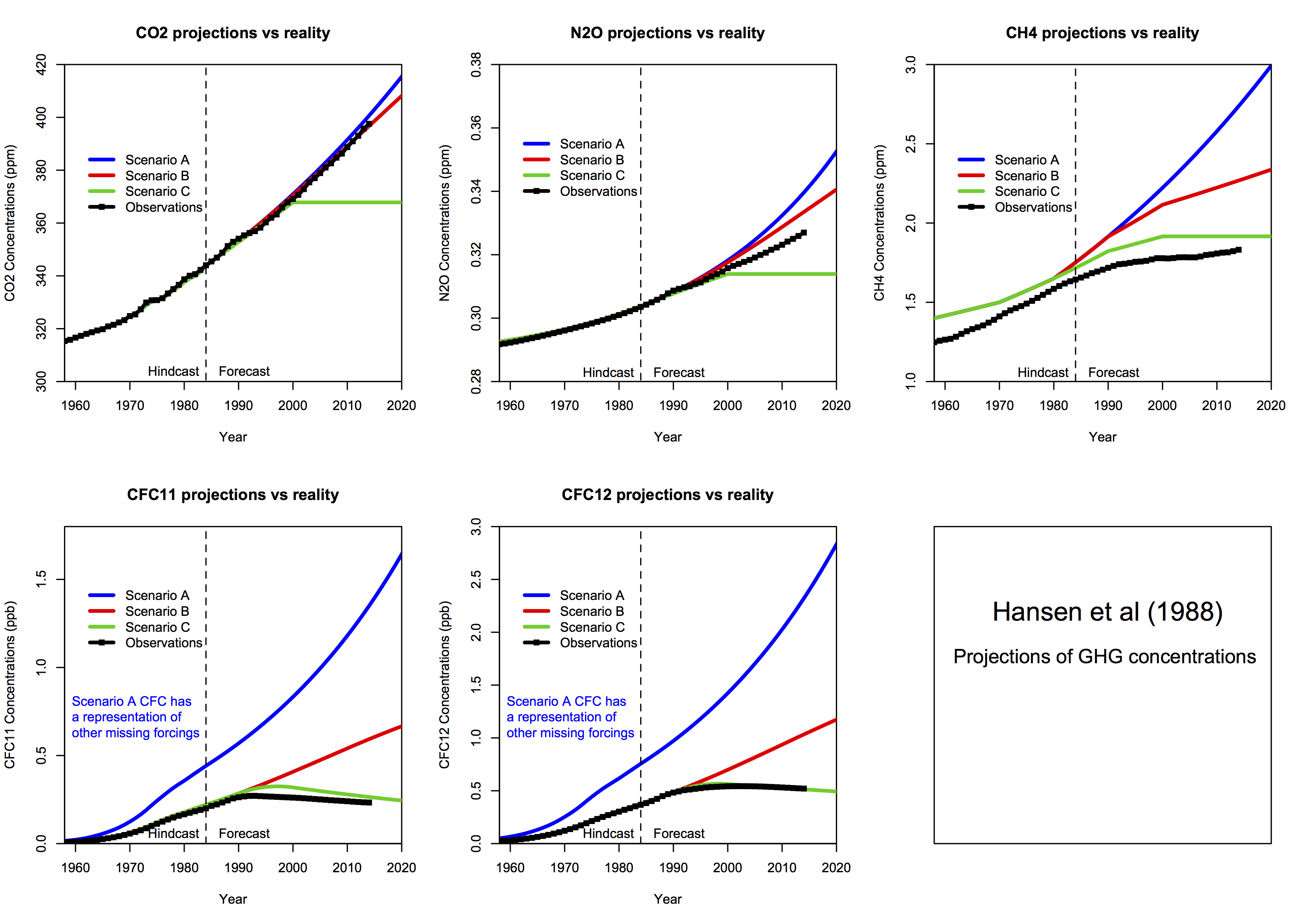
For comparison, Steve McIntyre showed graphs for his Scen_2, with data to 2008 only. There is no visual difference from scenario plots of Scen_1.
 |
 |
 |
 |
 |
Gavin also gave this plot of forcing, which demonstrates that when put together, the outcome is between scenarios B and C. This was also Steve McIntyre's conclusion back in 2008.
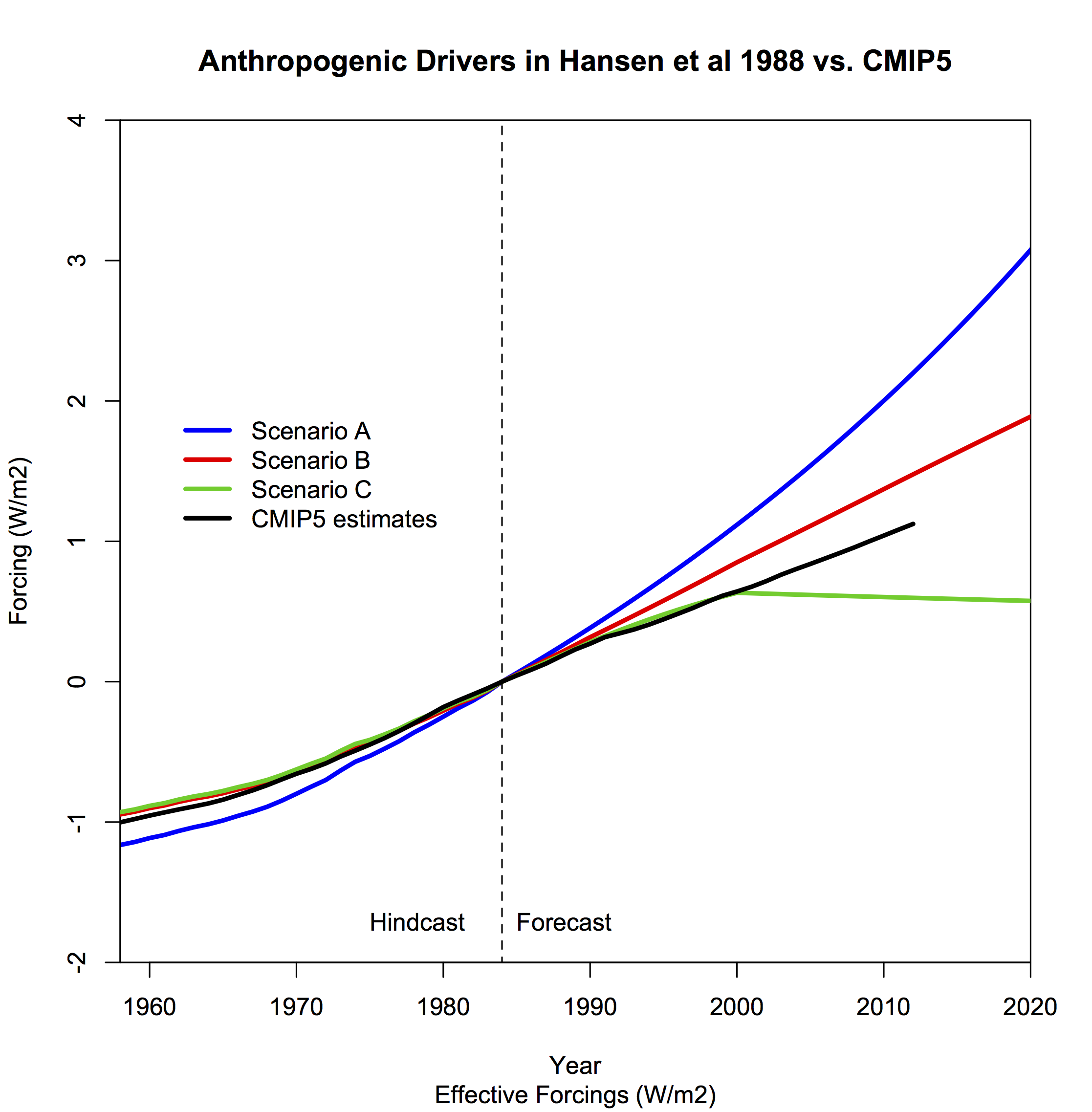
And here is another forcings graph, this time from Eli's posts in 2006 linked above (click to enlarge):


I sort of ran into the same thing with a denier over at ATTP's site with respect to Hansen's CO2 language ...
ReplyDeletehttps://andthentheresphysics.wordpress.com/2018/06/22/no-hansen-wasnt-wrong/#comment-125321
https://andthentheresphysics.wordpress.com/2018/06/22/no-hansen-wasnt-wrong/#comment-125325
https://andthentheresphysics.wordpress.com/2018/06/22/no-hansen-wasnt-wrong/#comment-125330
I already knew that emissions/concentrations themselves did not rise at 1.5% per annum (e. g. 1.5% of 180 ppmv (glacial) or 280 ppmv (PI) or 315 ppmv (circa 1958)). Hansen's language hinges on the words "annual increment" or "increment" (in ppmv) as you say for CO2. About 60 seconds in a spreadsheet showed me that Hansen's numbers, used correctly, are still remarkably close for today's aCO2 (~408 ppmv).
Willard was on hiatus (I guess) so I got the words knucklehead, dunce and stupid through with respect to said denier.
Everett,
DeleteYes, there has been a lot of it.
Went through this in 2008 with the same result
ReplyDeletehttp://rabett.blogspot.com/2006/06/business-as-usual-in-1988-more-silly.html
http://rabett.blogspot.com/2006/06/continuing-our-series.html
Thanks, Eli
DeleteI see it was even earlier, in 2006. I'll update the text.
I am cross posting an RR comment Nick, your thoughts are most welcome ...
ReplyDeleteI think that Hansen88 needs a forcing correction per ESRL AGGI ...
https://www.esrl.noaa.gov/gmd/aggi/aggi.html
https://www.esrl.noaa.gov/gmd/aggi/aggi.fig2.png
https://s3-us-west-1.amazonaws.com/www.moyhu.org/2018/06/gavin1.png
CO2 is close, between A and B
N2O is below A and B and above C (say ~ halfway between A and C)
CH4 is below C in its entirety
CFC11 is close to C but slightly below C for future projection
CFC12 is very close to C
Some groups include O2 (ozone) which gives a CO2e somewhere north of 500 ppmv today.
JC@CE has a post by McKitrick and Christy and they suggest not making the forcing adjustment ...
"Second, applying a post-hoc bias correction to the forcing ignores the fact that converting GHG increases into forcing is an essential part of the modeling."
Which actually supports making a forcing correction, use the forcing that actually happened, not Hansen's higher than actual forcing estimates. As the models are quasi-linear to begin with in the 1st place.
"Second, applying a post-hoc bias correction to the forcing ignores the fact that converting GHG increases into forcing is an essential part of the modeling."
DeleteThese guys don't know much. Converting GHG increases into forcing is not part of the modelling. You generally get the forcings by diagnosing model output. GCMs work with concentrations directly.
I've also been given the impression, by Gavin, several posts now, that the actual forcing to date are lower than the CMIP5 forcing as Gavin shows in this figure ...
ReplyDeletehttp://www.realclimate.org/images/anthro_h88_eff.png