NOAA GHCN station portal

NOAA has a rather unpublicized collection of visualisations of station data. I'll show Honolulu below the jump. It gives a visual summary of even monthly data, contrasts adjusted and unadjusted, including trends. You can enlarge in a new window.

Unfortunately, access seems to be only via an ftp directory in which the filenames are just number codes. Further it is broken into subdirectories which take a long time to load (just the filenames). So I thought I'd develop a portal. The one below is effectively just an extract of the inventory file, but with each station name linked  directly to its NOAA information.

I'm aiming to make something fancier with Javascript, to maybe select from a map etc. But the text version is a good start.

Update I'm glad to see the New NCDC has draggable graphs</a>. On looking further, I see they are using a service called multigraph.

Here is the station level information for Honolulu. It has been talked about lately because there has been recent decline, and in recent months the adjusted value has not been included. But it's actually of interest because the unadjusted data over the long term rises steeply, and the adjustment brings the trend down.



Now here is the list. As well as the station name and country, it shows the number of years of data, and the most recent year in which there is data. You can do text search (Ctrl-F) within the frame.

Nonsense with Illinois USHCN adjustments

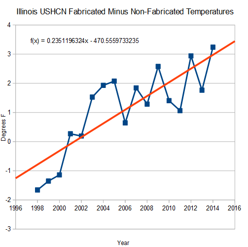
Zeke has been discussing USHCN adjustments and anomalies at Lucia's blog, specifically referring to Steve Goddard's continuing series of posts. SG has continued to get it wrong. Anyway, he bobbed up to point to this post, with the rather extraordinary claim that in Illinois, the adjustments make a difference of 23 °C/century (but only over the last 15 years). Zeke gave his own calc, which is quite different.

The claim is especially dubious because Illinois has a good record with fewer missing than USHCN generally, and his period is the last 15 years, relatively unaffected by adjustment.

So I did my own calc, using the code for the USCHN posts of here and here, but restricted to Illinois, where the 36 station numbers are from 110000 to 120000. I'll show plots below the jump. But this time I have no idea how he is getting it wrong, and he gives no code or detail. Illinois is much like USCHN, and there is little adjustment recently.



Here is SG's plot:



Here is my plot of the corresponding years.

F1-R1 is the correct way of calculating, averaging final-raw where both are known. SG-R1 is SG's method, where the average of all final, including interpolates, are differenced with the average of raw (a different set of stations). The red curve is the difference between green and blue. There is no big trend, as SG has, and the spread is much less.

Here is my plot of final-raw for the whole period. It corresponds to the whole USCHN story here

There is a spike in 2014, as explained earlier, caused by incomplete annual cycle, and some trouble before 1900. Otherwise very similar.

This time I have no idea where he has gone wrong.

Detecting periodicity

I've been following, and occasionally joining in, a series of threads by Willis Eschenbach at WUWT. Here is the latest, and you can follow links back.

Willis is trying to detect periodicity in various segments (century or so) of monthly or annual data. Lately he has been trying to decide whether sunspot (SSN) periodicities can be observed in climate data. This involves first establishing the major periodicities in SSN, and then looking at periodicities in signals which might be responding.

In the early part, Willis was fitting sinusoids using a least squares fit by optimisation. In this comment, I showed that the quadratic form could be expressed as a fairly orthodox discrete Fourier Transform expression, and wrote code to show how the same result could be derived. Willis then recharacterised what he was doing as a Slow Fourier Transform; here I try to put that in context.

I was not, BTW trying to suggest that what Willis was doing was wrong; only to say that it could be done more efficiently by FFT methods (which involved padding), and there was a long history. In fact someone characterised it as a Lomb periodogram, and it is certainly of a class of Least-squares spectral analysis (LSSA).

In the most recent version, he is using regression of the data onto sinusoids, and investigating the effect of using monthly or annual time divisions. Tamino chimed in in a positive spirit (the thread was called "Well, Color Me Gobsmacked!"), and said the method was known as the Date-Compensated Discrete Fourier Transform.

I think Willis now regards the chief advantage of the method as allowing for irregularly spaced data, in his case missing months, and that is what the DCDFT is for.

The method is sometimes being criticised as not being a truly orthogonal decomposition. I think that is misplaced. You can look for periodicities in a Fourier decomposition, but it is not the only way. I think Willis is basically filtering. He creates the equivalent of a perfectly tuned circuit, which takes the data as input, and identifies the amplitude of the response as the measure of periodicity. I think that is fine, and so I'd like in this post to say how one might assess and maybe improve the merit of that measure.

It's like what you did with the old AM radio receiver. By frequency shifting with a knob, you listened to the sound level to find stations.

What I want to do in this post is to show how you can get past all the issues of missing data and orthogonality, and rephrase in terms of Fourier integrals, which exposes the sources of error. I'm expanding on this comment.

Willis' method as a filter

For any given frequency ω, Willis uses the R lm() function to fit a+b*cos(ωt)+c*sin(ωt). He then returns √(b²+c²) as the amplitude of the fitted sinusoid. He usually plots this against period, not frequency, and looks for peaks.

This is a linear filter on the input. Normally we think of a filter as modifying one time series to another. This is a perfectly tuned filter, in that it produces a pure sinusoid as output. That is rather boring, in that it can be characterised by two numbers, amplitude and phase, and Willis drops the phase. But it is still a filter. You can think of it as a tuned circuit (or bell or cavity etc) which responds to frequencies near its resonance.

Expression as an integral

I'll assume that the data represents samples from a continuous function f(t). This assumption is basic to any continuum analysis. You have to assume that the data you have is representative of the values in between. f(t) could, for example, be a linear interpolate.

The sum Willis is evaluating in lm() can then be expressed as an integral:
∫ Ψ(t) cos(ωt+θ) f(t) dt
ω is angular frequency, θ phase.  All integrals here are from -∞ to ∞, but Ψ(t) is sum of a finite number of delta functions. I've chosen Ψ to suggest a shah (Ш) function, also called a Dirac comb of delta functions. Generally it will here be mostly equally spaced, but that is not a requirement. It is truncated.

So now we can see what kind of filter it is, by looking at the Fourier Transform. The FT of cos is just a paired delta function that shifts the spectrum of Ψ(t) to center on ±ω. So if Ψ has, say, N=200 delta functions with s=1 annual spacing, the Fourier transform (t origin at the middle) is
sinc(Nω)/sinc(sω)
where sinc(x)=sin(x)/x

It looks like this in the frequency domain:

and the amplitude looks like this:


It is symmetric about 0. When combined with the sinusoid, it is displaced. Willis is looking for periods around 10 years; using that as a test frequency gives:



I think this shows a number of things. There is a peak at 1/10 yr^-1. It has side lobes, which represent the effect of the finite (200 yr) interval. These affect the ability to discriminate peaks.  It is actually periodic overall, with period 0.5 yr^-1 (the FT alternates in sign and  has period 1 yr^-1). That shows problems when you get up to the Nyquist frequency. But the peaks are fairly sharp, and the Nyquist troubles far away, at least if you are looking at periods of 10 years or so.

Irregular points

The sinc function ratio is actually the sum of sinusoids evaluated at the sample points. You can evaluate at a set less regularly spaced, with missing values say, and the function won't be radically different. And of course, the method still works.

Other ideas

In recent discussion, I've put some other analogies. The method is actually like the way analogue spectral analysis was done. Tuned circuits, acting as filters, responded to the signals in a tuned way. If you aren't familiar with circuits, think of a bank of lossless tuning forks, mounted on a sounding board, say. You buzz the burst of signal, and see which ones pick up the most energy.

The mathematics of the regression Willis uses is in fact the math of heterodyning. You multiply by a sinusoid and add. If the signal can reasonably be fitted with a nearby sinusoid, then the trig formula for products will yiekd a beat frequency, lower in pitch as the two frequencies are closer. The addition is a low pass filter, passing with amplitude inversely proportional to frequency. So its response is approximately proportional to both the strength of the periodic component, and to its closeness.

What next

I'll stop here for the moment. I'd like to deal with the effect of annual averaging, which fits in nicely, and was one of Willis' topics. I'd also like to deal with the effect of windowing, with the idea of making the side lobes diminish faster. I think it will help, but the current situation isn't bad.

Anomalies.

This is a followup to my two previous posts (here, and here). In the last, it was shown that in comparing two different USHCN sets (raw and final) a spike in 2014 was due to the data coming from different periods. The spike was there even if the climatology was substituted; so it wasn't a result of actual 2014 readings, only when and where they happened.

Now I'd like to draw some lessons from that in terms of anomalies.

1. How anomalies remove the spike.
   
2. How they allow comparison of disparate multi-year data in global indices
   
3. Why anomalies are expressed on fixed base intervals, and
4. How this might be improved.
   

The USHCN adjustments spike

Averaging is linear, and you can think of it as applied to the sum of an expected value (climatology) and an anomaly (the information part). If the expected value is subtracted, the cause of the spike goes away. Put another way, if the expected value is near zero, it won't matter much if the station/months in the samples vary. Let's see how that works.

 For each station/month, I'll subtract the longterm annual raw average. That is, from a May reading, I'll subtract the May average. Here are the equivalents of R1, F1 and SG from the previous posts.

 It corresponds to this plot from the previous post; 2014 has no spike and has not been omitted. You can see that it is broadly similar except for the offset. But now F2 (the average of unmatched final data) is far less out of line, and so the mauve SG (average of all final) is very close to F1 (average of matched final). SG's method, mine all give much the same.

Missing values - infilling

In this post I showed how for a fixed grid with empty cells, you could say that averaging with missing values and averaging with missings infilled with the average of what was there gave the same result.

This is true for subset averaging. If you average first over latitude bands, it's equivalent to infilling with the subset average. That gives a criterion; the averaging should be done so that the infill is closest to your expected value. So latitude band averaging is better, because there is a systematic latitude effect on trend.

 When comparing two different sets, with no natural set of slots for data, missing means unmatched. If there are station/months in one average but not the other, the latter can be treated as missing, and considered infilled by average.

 You could try to improve with explicit infill. But if you have a time series plot, say, the missings between any pair are different. So explicit infill won't work. But you can offset so that each average is of points with as near as possible zero expected value. Then the default infill is near zero. That's the anomaly approach.

Global indices

These are compiled from a scatter of stations with very different reporting periods. These are conventionally assembled into grid cells, anomalised and the cell averages averaged. This compensates for variations in station density. But if the cells are small enough to give good resolution, then many will be empty.

 It is also possible to make station anomalies directly by subtracting long term month averages. Then some suitable spatial integration formula is needed.

 The inter-set comparison logic is needed just to make the time series coherent - you can compare any pair of years and know they are on the same basis. You aren't seeing big differences because stations drop in or out. A famous example where this didn't work so well was the Marcott spike.

 You can extend the concept of missing data to cover all points that aren't sampled. Again there is implicit infill. You can see this in two ways. The quadrature formula brings weights, so it's equivalent to infilling with a weighted average. Alternatively, the quadrature is based on forming and integrating a local interpolate. These two ways should be consistent.

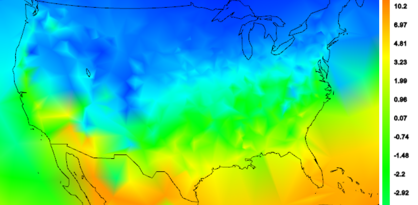
 I'd like to show the effects of various anomaly methods. First here is a shaded plot of absolute temperatures for US April 2014. This is unadjusted min/max average for GHCN stations (QCU). There is a strong latitude variation, which dominates the local variability due to altitude. The color scale is actually a cut-off fragment, and is also non-linear. But you can see how the average might vary depending on how evenly the stations sample the latitude zones.

 

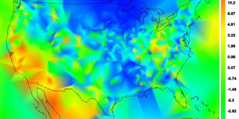
 Now here is a shaded plot of individual US anomalies for April 2014, calculated just as differences from the long term mean of all April data. The latitude dependence is gone, but it is fairly blotchy, empohasised by the way the triangular mesh does shading. In these plots, the colors are correct for the actual stations, and linearly shaded in between. The blotchiness is partly due to the fact that some stations have long records, and so a fairly low average, because of the cooler past. Low average means high anomaly. Others have only recent data and a higher average.

 

Common basis years

There is a catch. Using long term averages which are typically all available data removes variation in station climatology and seasonal monthly. But there may be a secular variation over years - probably a trend. You'd like to know what that is.

However, it also means that the flat mean is not the best estimate. There will again be a bias in that stations whose anomaly mean is formed with more recent data will have a lower expected anomaly that those who don't, so again it matters what stations are in the mix.

 The standard remedy is to choose common base years, eg 1961-90, for each station/month base. But then there is the problem of stations lacking data in the period.

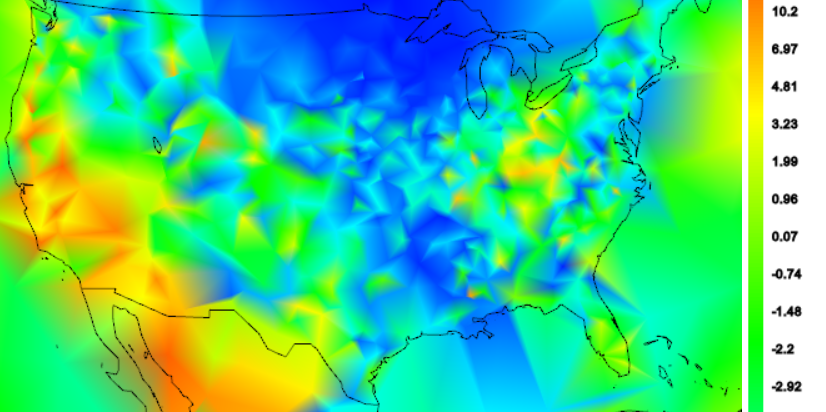
 In the next plot, I've used a trick to overcome this. I've used an exponentially weighted linear trend fit. The weight is centred at 1975, and gives most weight to data in the range 1961-90, which is a common choice for anomaly base interval. I use the 1975 intercept. In that way I can get a reasonable estimate even if there is data missing in that interval. It won't work so well for stations that stopped long before, but they won't have 2014 values anyway. GHCN has few if any US stations that started post 1975.

 

 You might agree that it is better than averages taken at whatever time there is data; it takes out that variability. But it still has variability due to variation in trend since 1975.

 Another way is to detrend completely. That is the standard way of removing expected value. But the trend is wanted, so has to be recovered after averaging.

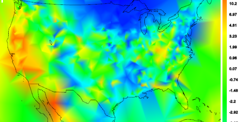
The next plot shows the April 2014 plot where each station has been locally detrended, again with exponential weighting. You can see that as each element of expected value is taken out, over the succession of plots the map gets (slightly) smoother.

 

Conclusion

Anomalies represent an attempt to romove as much as possible from a signal that is predictable, generally prior to averaging. Since the residuals have much reduced mean, there is less sensitivity to variation of stations/months in the sample.


Since the part removed reflects non-climate variations like topography, latitude and seasonality, the remainders have a better chance of showing whatever coherence there is in the information part. Hence the improving smoothness. It gives a better chance that the samples will reflect the measurand in between locations.

USHCN, adjustments, averages, getting it right.

There has been quite a kerfuffle about USHCN adjustments. There was a WUWT post on reasons for the spike, a recalc at Steven Goddard's site, and more here and here. But the basic elementary issue is little understood. You need to be very careful doing arithmetic with averages of data from disparate situations. I'll show why.

I introduce three annual averages. F1 and R1 are averages of Final and Raw USCHN data over just the set where both numbers are known. Then F2 is the average of Final, in each year, over data where the raw is not known.

My earlier calculation was F1-R1, or equivalently, the average difference between final and raw when both are known. This is clearly a measure of adjustment. Steven Goddard's variants all include F2 in some way. I'll show that this is never helpful, and leads to silly results.



First, a simple rule for combining averages. If you have a set S of N numbers, made up of subsets S1 (N1) and S2 (N2), and the respective averages are A, A1 and A2, then
A=p*A1+q*A2, where p=N1/N, q=N2/N and p+q=1
{Proof N*A=N1*A1+N2*A2)

In averaging USHCN data with adjustments, we have in each year a set S1 of N1 station/months that have both raw and final data, and a set S2 of N2 that have final alone. Call F1 and R1 the averages of final and raw on S1, and F2 the average of final on S2.

Caveat: I have started from 1900 from where it is almost true that all stations have final data. There are just a few (max 3) missing in some years of the first decade. I believe that makes no difference to the analysis.

Steven Goddard (SG), took the average of all raw from all final:
A_S = p*F1 + q*F2 - R1 = (1-q)*F1 + q*F2 - R1 = (F1 - R1) + q*(F2-F1)
I took the averages of differences where they exist, which is exactly:
A_N = F1 - R1

So A_N is indeed an average of known adjustment differences. SG has combined it with something else. What does that achieve?

SG insists that it adds, or retains, information about the interpolation (F2). But we don't have a difference between interpolated and raw. Instead, he has combined it with F2-F1, which is the difference between two sets of final values.

This really makes no sense. But it led to the "spike". The reason is that the interpolated points are more frequent in the latest month, April. And that is the warmest month. While R1 is on the complementary set, which is the cooler period. The small adjustment makes little difference here, compared to seasonal. In fact, for recent years, raw and adjusted are virtually identical.

I'll illustrate. I'll start with a plot of p, the fraction of stations reporting. For a long time it was almost one. In the early part there is more loss, and since 1990 the number of active stations has reduced. There is a sharp dip in 2014, because some data comes in late; this mostly affects the most recent month. (Actually, the dip is exaggerated in the plot because it counts May-Dec 2014 as missing)



Now here are the three data average sequences, R1, F1, F2; everything else is a linear combination of them:



The downspike in 2014 is due to being mostly winter so far; a caution of troubles to come with absolute temperatures. The next plot is smoothed (7 year MA) to compare with the SG plot here, where "Raw" is R1 and "Final" is A_S, which I've called SG (average of all final)SG. The "new method" there is averaging by months first which makes a big difference for 2014, but else not. More later on that. Here I've removed 2014.



SG claims that the adjustment turns the downtrend raw R1 (blue) into the uptrend SG (purple). I think the right comparison is with F1 (red). It actually doesn't make a big difference in the midrange, where there is little missing data. But at the ends it does, and SG exaggerates the uptrend produced by adjustment.

Those are absolute plots. Next I'll subtract R1 from F1 and SG, and also show the difference curve. We agree that R1 is the right measure of "raw".



The green SG-R1 was the original spike plot shown at WUWT. The blue F1-R1 was my corrected version. Again you can see that they track mid-range, but diverge near the ends, giving SG-R1 a much greater range. The red curve is the extra bit that he has included. You can see that the difference generates the spike. The reason is that in F2-F1, April has a lot more missing raw values than other months. So F1 is a much more wintry set of data than F2.

I've contended that introducing F2-F1, via SG, makes no sense. Steven Goddard obstinately disagrees, claiming that he's preserving something about the final adjustments. The next plot puts this in perspective. I compare that inclusion with what you get if you do the same calc with data that is just the climatology - ie the average raw temperature, for each month, but constant over all years. I've called that Z, and like F it breaks into Z1 and Z2 on S1 and S2. This has no information about the annual weather, or the adjustments



It shows that almost all the introduced term F2-F1 is accounted for by the variation in the climatology - ie different kinds of stations reporting for each month. Between months matters more than between stations, because of seasonality which is a systematic shift for all stations. The green curve is what you get after multiplying by q, and would be the same for q*(F2-F1). But that is exactly the difference between SG's curve and mine.  And it shows clearly the 2014 spike, which is entirely predictable from knowing average (not 2014) temperatures only.

Averaging months first

As mentioned above, SG has an updated method. He gets the annual average by averaging the data for each month first, and then by year. You might think that shouldn't matter, and the fact that it does is a bad sign. It makes little difference to F1-R1, the correct measure. But it does to the added F2-F1.

We might as well think about this as generating a monthly plot, which can then be binned to annual. It removes the spike because F2-F1 is now evaluated on the same month. Each month is weighted equally.  But there is still the difference due to the stations reporting having on average warmer or colder climates than those that don't. Maybe by luck they will be the same. But there's no reason to rely on it. There's nothing to gain, and accuracy to lose. Here is the comparison of the difference and the climatology only version, worked out that way:



Again the green curve is what is added, and has smaller scatter, so when added to F1-R1 it makes less difference (still some spike, though). But again, it's almost exactly what you get calculated by climatology. It adds no information about temperatures, nor adjustments. It's just error.

Where next?

I've spent a lot of time on this case because I think it helps get thinking on averages straightened out. It helped me. I also think it's worth getting the calculation of the effect of adjustments right. There are effects, and they do have in total an uptrend effect. That's the way it is. But there is no need to bewail the way it isn't.

I'll write more on averaging and temperature indices. It was the basic issue that Cowtan and Way found with HADCRUt 4. The issues are non-trivial.

April GISS Temp up by 0.03°C

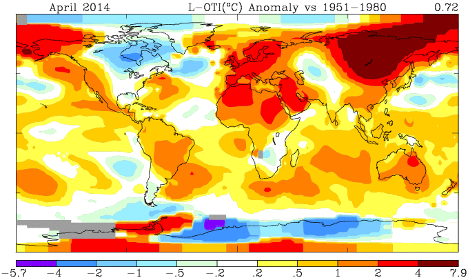
GISS has posted its April estimate for global temperature anomaly, and like TempLS it showed a small change, rising from 0.70°C in February to 0.73°C in April. That's getting quite high.

The comparison maps are below the jump.

Here is the GISS map:



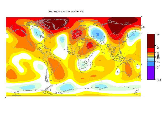
And here, with the same scale and color scheme, is the earlier TempLS map:


It shows the same cool in N Central N America, and central Asia and rather warmer in E Asia. It doesn't show the TempLS warmth in Greenland, which as I warned was likely an artefact of the lack of readings there..

Previous Months

March
February
January 2014
December
November
October
September
August
July
June
May
April
March
February
January
December 2012
November
October
September
August
July
June
May
April
March
February
January
December 2011
November
October
September
August 2011

More data and plots

TempLS global temp stable in April

TempLS showed a very small rise in April; from 0.618°C to
0.619°C. The satellite indices showed little movement.

Again I had to remove some suspect readings, which I've noted here. Here is the spherical harmonics plot:



Still cold in Great lakes and N, and Central Asia. Warm in W Europe. The warmth in Greenland may be exaggerated by the removal of suspect station data.

Here is the map of the 4255 stations reporting: