Rising Trends

About a month ago, I wrote a post about how trends of global temperature calculated over recent past periods had been rising, and the periods of zero or negative trend, commonly quoted as evidence of the "pause", were likely to diminish rapidly if warm weather continued.

The weather has been warm, and with another month of data, that process has continued. I'll show the active plot below, in which you can see how the trends calculated over various periods back from now have changed since March, and are likely to change in the next three months if current warmth continues.


There has been a change to HadCRUT data since the last report. A new version of HadSST3 caused subsequent changes in HadCRUT4. I believe that are also fewer empty cells in HadCRUT4, which will help remove the cooling bias that Cowtan and Way identified. The changes to both HadSST3 and HadCRUT4 are noticeable.

In the active plot below, you can use the arrows to cycle through the months from March to November. Future data is padded by reflection - September is the same as August, October as July etc. In fact we have data for MSU and UAH in September. MSU was about the same, UAH a bit higher. I stuck with the padding for this post.

As before, what is plotted is, for each date, the trend of temperature from that date to August 2014. Of interest for pause talk is where the curves cross the x axis.

Analysis of short-centered PCA

There has been a lot of to and fro (see recent posts) about short-centered PCA - MBH style (background). My general view here is that there is an effect on the first principal component, but that merely moves to a particular alignment of basis vectors, and doesn't affect any reasonable reconstruction. And it all happened so long ago...

But still it's an interesting analytic problem, so I did some analysis. It particularly concerns the role of persistence, or autocorrelation. Increased autocorrelation tends to show more effect, because for a given number of proxies, it diminishes the effect of noise relative to the underlying short-centering operator (graphs below). But that underlying pattern is interesting, because it is much less dependent on autocorrelation. And the next PC's in succession are interesting, as I wrote about here.

White noise

You need an infinite quantity of proxies to see a pattern with white noise. But the pattern is the prototype for more difficult cases, so I'll develop it first. Much of what I have done recently is based on the work in the NAS report and its associated code. They compute and scale not only PCA first components from AR1() proxies, but also from the associated correlation matrices, which they scale and put on the same graph.

The algebra of short-centered averaging works like this. Define a N-vector h which has zeroes outside the short averaging period (M years at the end of N years of data), and values 1/M within, and another vector l which has 1's only. Then for a data vector x, length N, the valkue with short mean deducted is x-l*(h.x), or E*x, where E=I-l⊗h. I is the identity matrix, and ⊗ the dyadic product. For future reference, I'll note the dot products
l.l = N, l.h = 1, h.h = 1/M.

Then for a data vector X, Nxp, p the number of proxies, the PC's are the eigenvectors of XX^*. The expected value of this, as a random noise vector, is p*K, where K is the autocorrelation matrix. For eigenvectors we can drop the p. The short-averaged version is E*X*X^**E^*. So for white noise, K is the identity I, and we need just the eigenvectors of E*E^*.

Expanding, the eigenvalue equation is
(I-l⊗h - l⊗h + l⊗l h.h)*u = z u
or
(l⊗h + l⊗h - l⊗l h.h) u = (z-1) u

Since the matrix on the left now has range spanned by l and h, u must be in this space too. So we can set u = A*h+B*k, and there is a 2-dim eigenvalue for u in this space. I'll skip the 2-d algebra (just substitute u and work out the dot products), but the end results are two eigenvalues:
z=0, u=l
z=N/m, u= l-h
The latter is clearly the largest eigenvalue. There are also a set of trivial eigenvalues z-1=0; these correspond to the remaining unchanged eigenvalues of I.

So what has happened here? The short averaging has perturbed the correlation matrix. It has identified the vector u=l-h, which is 1 for years in 1:(N-M) and zero beyond, as the first principal component. This will appear in any reduced set of eigenvalues. All vectors orthogonal to it and l are still eigenvectors. So no new eigenvectors were created; u had been an eigenvalue previously. It just means that now whenever a subset is formed, it will come from a subset of the unperturbed set. They were valid bases for the space before; they still are.

Effect of autocorrelation.

I showed earlier DeepClimate's rendering of two AR1() cases from the NAS code:

AR(r=0.2), 5 PC1s from sets of 50 proxies.	AR(r=0.9)

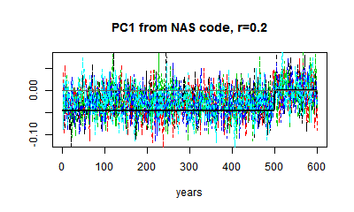
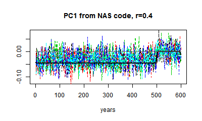
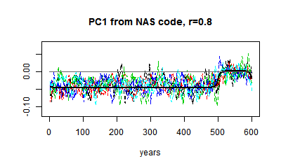
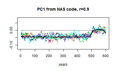
You can see that relative to the HS effect, the noise is much greater when r=0.2 (it depends on proxy numbers). And I can't usefully show white noise, because the noise obliterates the effect. but the eigenvector is not very different.

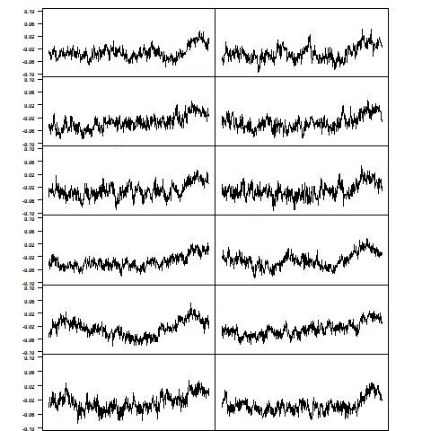
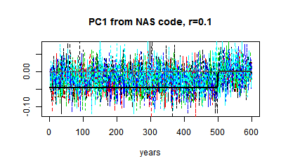
Here are some plots of PC1 from r=0.1 to r=0.9. I've kept to the same scale. You can see the gradual change in the matrix eigenvector, and the gradual downscaling of the noise, which makes the eigenvalue pattern stand out more.

Next

My main ambition here was to get theoretical expressions for these eigenvalues. It is possible, and interesting, to convert the eigenvalue equation to a difference equation, which emphasises the Sturm-Liouville pattern for higher eigenvectors. For PC1, it just gives an expression for the rounding that you see. That's for another day.

What Steve McIntyre won't show you - now

but he did once. It's what the end effect is of all these interminable claims about mining for hockey sticks etc. What it actually does to a reconstruction.

Update 
Steve McIntyre has taken exception to this post, with his own post entitled Sliming by Stokes. He has claimed in the comments here that: 

"Stokes’ most recent post, entitled “What Steve McIntyre Won’t Show You Now”, contains a series of lies and fantasies, falsely claiming that I’ve been withholding MM05-EE analyses from readers in my recent fisking of ClimateBaller doctrines, falsely claiming that I’ve “said very little about this recon [MM05-EE] since it was published” and speculating that I’ve been concealing these results because they were “inconvenient”." 

I've responded in a comment at CA giving chapter and verse on how he avoided telling the Congressional Committe to which he testified, which had a clear interest, about these inconvenient results. So far, no response (and of course no apology for the "sliming").

That was shown in MM05EE, their 2005 Paper titled:
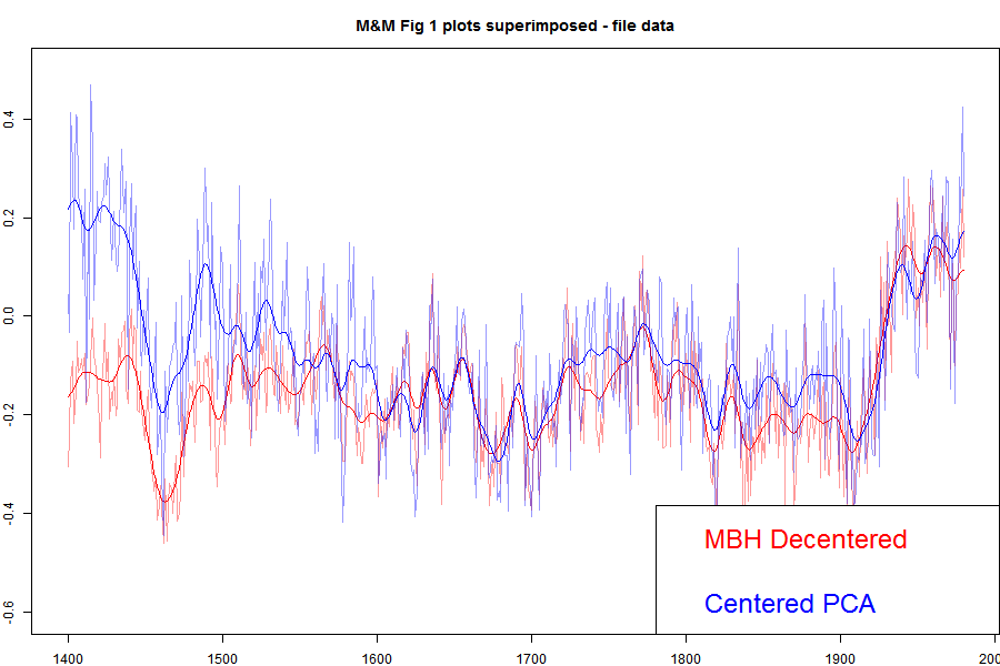
"The M&M critique of the MBH98 Northern Hemisphere climate index: update and implications". I've shown that plot in an appendix here, and I'll show it again below. But for here, I'll show the plot with the MBH decentered and M&M centered superimposed.



Update: When I printed out the data from my running of the MM05 code for Carrick below, I noticed discrepancies between the numbers and the emulation.txt data on file. I've tried to track down the reason, but I think the simplest thing to do is to switch to using the emulation.txt data directly, which I've done. The MBH and the corrected still track closely in recent centuries, but there is a somewhat larger discrepancy in the 19th century. Prvious versions are here and here..
The agreement is very good between, say, 1800 and 1980. These are the years when all the alleged mined hockey sticks should be showing up. They aren't. There is a discrepancy in the earlier years, which DeepClimate explains here. When Wahl and Ammann corrected various difference between the M&M emulation and MBH99 (in their case) this early period discrepancy disappeared. But anyway, for now what is important is that both centered and uncentered agree very well in the period where decentering is supposed to be mining for hockeysticks. Steve Mc has said very little about this recon since it was published, so much so that when Wegman was pressed (properly) by Rep Stupak at Congress on why he hadn't shown the results of a corrected calculation, he had no good answer, and didn't refer to M&M2005, even though he was supposed to be familiar with the code (which he had) which did it. I think this has become a very inconvenient graph.

I described earlier how apparent PC1 alignments have an effect on reconstruction that disappears rapidly as more than one PC are used. I'll give below a geometric explanation for this, which explains the irrelevance of MM)5 fig 2, which resurfaced as Wegman's fig 4.2.

Here is the plot direct from MM05EE. The bottom "centered" includes the removal by M&M of the Gaspe cedar data from 1400-1450, which affects those years.



I've described the Gaspe issue, with some more plots here.

With trouble over the 100/1 sampling, Steve McIntyre has promoted his histogram, which appeared as Fig 2 in the MM2005 GRL paper, and as Fig 4.2 in the Wegman Report. The present re-presentation as a t-statistic adds nothing.

I've explained any times how all PCA is doing here is realigning the axes so that PC1 aligns with HS behaviour. In the simulated case, without that the axis directions are not strongly determined, and with white noise, not determined at all. That last means that all possible configurations are equivalent and would give the same results in any analysis. It takes only a slight pertuebation for one alignment to be preferred - how strongly depends on the randomness, not how much difference the alignment makes. I used the following analogy at CA:

"Let me give a geometric analogy here. Suppose you live on a non-rotating spherical earth. You want a coordinate system to calc average temperature, say. You want that system to have a principal axis along the longest radius. You send out teams to measure. Their results have no preferred direction. There is a Pole star, so you histogram a Northness Index. It looks like the first one here. A sort of cos.

Now suppose the Earth is very slightly prolate, N-S, but the limit of measurement. Your teams will return results with a N-S bias. Your histogram of Northness will lbe bimodal like the second above. The spread will depend on how good the measuring is relative to the prolateness. If measurement is good, there will be rare few values, and the two peaks will be sharp.

The definiteness of the histogram has nothing to do with whether alignment of the principal axis matters."

Again there is no evidence that any aspect of Mann's decentered PCA has ever affected a temperature reconstruction, despite all the irrelevant graphics about PC1.

Update. Here is the corresponding emulation from Ammann and Wahl. There is now no large discrepancy in the earleir years.


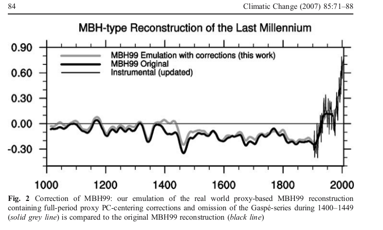
Update: DeepClimate, in a comment here, has linked to the plot below, which shows just how far MM2005 deviated from the MBH recon with centered mean - this time shown against the millenium recon.

Update: Pekka has added a comment which I reproduce with diagram below:

Pekka Pirilä October 8, 2014 at 9:00 AM
As this issue has been discussed so much, I wanted to understand it better and reproduced four variations of PCA of the NORAM1400 network:

1) short-centered MBH98
2) scaling as in MBH98, but fully centered
3) standard scaling and centering
4) without scaling of the original time series (MM05)

Otherwise the results are as reported elsewhere (e.g. in Wahl and Ammann, 2007), but I added the comparison of, how much each PCA explains by up to 10 first PCs calculating the shares from the real variability of time series used in each analysis. Thus the shares are calculated from the same total variance in cases (1) and (2), from slightly different in (3) and from substantively different in (4) where the variances of individual time series vary greatly.

The results are shown here



What many may find surprising is that my numbers for MBH98 are very different from those shown in several places (e.g. RealClimate). The reason is that those numbers are not based on the variability of the time series, but on variances around the short-centered mean. That adds both to the total variance and to the contributions from individual PCs. In relative terms it adds much more to PC1 than to the total. Thus the resulting number does not tell about the real variability, but is very much affected by the decentering.

I calculated my values by first orthonormalizing the basis relative to deviations from full mean (the mean affects, what's orthogonal), and by using this orthonormal basis for determining, how much the space spanned by N first PCs of the MBH98 analysis can explain.

More ClimateBall at Climate Audit

Steve McIntyre has a new post up at ClimateAudit. It's called "What Nick Stokes won't show you". It's a continuation of the smokescreen about demanding the unselected PC1s be shown with orientation favorable to a hockey-stick interpretation, using a hockey stick index (HSI), rather than as his program produces them. Again pretending that it's about Wegman aligning the orientation, rather than selecting the top 1% by HSI without disclosure.

He's made some pretty outrageous claims about how people here are, well I'll quote: "Some ClimateBallers, including commenters at Stokes’ blog, are now making the fabricated claim that MM05 results were not based on the 10,000 simulations reported in Figure 2, but on a cherry-picked subset of the top percentile. "

I wrote a substantive response to this, soon after the post appeared. It went into moderation - I've posted the text here. About four hours later it disappeared from the queue; I don't know what is happening there. Steve says he'll look in the morning. (It's here).

I reran the code to get some quantitative HSI numbers for the various cases, matching those described in detail here, and pictured here. It's a new run, not exactly matching. Here are the numbers, matching the cases described . For unselected sets, it's the mean absolute value HSI:

	Decentered PCA (MBH98)	Centered PCA
Selected 100 out of 10000 by HSI	1.98	1.60
Not Selected	1.61	0.65

The mean of 1.61 for unselected decentered (MBH) matches the mid-range figure in Steve's post. The difference between 1.98 and 1.61 made by selection may not seem so great, but these are like t-values. And it shows when centered but selected has almost the same mean HSI. The undisclosed selection is about as effective in creating HS appearance as decentering.

Emphasising the compression of the t-like HSI scale, centered unselected, which shouldn't have any HSI effect, and don't seem to, still show a mean (absolute) HSI of 0.65.

Anyway, below the jump I'll show various plots relevant to Brandon's contention that they should be oriented.
Here is the original Wegman tableau:


It is the selected version, with a mean HSI of about 1.98. I contrasted it with an unselected version. Brandon modified this to show the plots with positive HSI:

post up at ClimateAudit. It's called "What Nick Stokes won't show you". It's a continuation of the smokescreen about demanding the unselected PC1s be shown with orientation favorable to a hockey-stick interpretation, using a hockey stick index (HSI), rather than as his program produces them. Again pretending that it's about Wegman aligning the orientation, rather than selecting the top 1% by HSI without disclosure. He's made some pretty outrageous claims about how people here are, well I'll quote: "Some ClimateBallers, including commenters at Stokes’ blog, are now making the fabricated claim that MM05 results were not based on the 10,000 simulations reported in Figure 2, but on a cherry-picked subset of the top percentile. " I wrote a substantive response to this, soon after the post appeared. It went into moderation - I've posted the text here. About four hours later it disappeared from the queue; I don't know what is happening there. Steve says he'll look in the morning. (It's here). I reran the code to get some quantitative HSI numbers for the various cases, matching those described in detail here, and pictured here. It's a new run, not exactly matching. Here are the numbers, matching the cases described . For unselected sets, it's the mean absolute value HSI: Decentered PCA (MBH98)         Centered PCA Selected 100 out of 10000 by HSI      1.98 1.60 Not Selected 1.61 0.65 The mean of 1.61 for unselected decentered (MBH) matches the mid-range figure in Steve's post. The difference between 1.98 and 1.61 made by selection may not seem so great, but these are like t-values. And it shows when centered but selected has almost the same mean HSI. The undisclosed selection is about as effective in creating HS appearance as decentering. Emphasising the compression of the t-like HSI scale, centered unselected, which shouldn't have any HSI effect, and don't seem to, still show a mean (absolute) HSI of 0.65. Anyway, below the jump I'll show various plots relevant to Brandon's contention that they should be oriented. Here is the original Wegman tableau: post up at ClimateAudit. It's called "What Nick Stokes won't show you". It's a continuation of the smokescreen about demanding the unselected PC1s be shown with orientation favorable to a hockey-stick interpretation, using a hockey stick index (HSI), rather than as his program produces them. Again pretending that it's about Wegman aligning the orientation, rather than selecting the top 1% by HSI without disclosure. He's made some pretty outrageous claims about how people here are, well I'll quote: "Some ClimateBallers, including commenters at Stokes’ blog, are now making the fabricated claim that MM05 results were not based on the 10,000 simulations reported in Figure 2, but on a cherry-picked subset of the top percentile. " I wrote a substantive response to this, soon after the post appeared. It went into moderation - I've posted the text here. About four hours later it disappeared from the queue; I don't know what is happening there. Steve says he'll look in the morning. (It's here). I reran the code to get some quantitative HSI numbers for the various cases, matching those described in detail here, and pictured here. It's a new run, not exactly matching. Here are the numbers, matching the cases described . For unselected sets, it's the mean absolute value HSI: Decentered PCA (MBH98)         Centered PCA Selected 100 out of 10000 by HSI      1.98 1.60 Not Selected 1.61 0.65 The mean of 1.61 for unselected decentered (MBH) matches the mid-range figure in Steve's post. The difference between 1.98 and 1.61 made by selection may not seem so great, but these are like t-values. And it shows when centered but selected has almost the same mean HSI. The undisclosed selection is about as effective in creating HS appearance as decentering. Emphasising the compression of the t-like HSI scale, centered unselected, which shouldn't have any HSI effect, and don't seem to, still show a mean (absolute) HSI of 0.65. Anyway, below the jump I'll show various plots relevant to Brandon's contention that they should be oriented. Here is the original Wegman tableau: It is the selected version, with a mean HSI of about 1.98. I contrasted it with an unselected version. Brandon modified this to show the plots with positive HSI: Unselected, as produced by MM05 program As reoriented by Brandon He says that it makes a big difference. Judge for yourself. But is it a legitimate difference? It makes any kind of trend look like a HS contribution, by turning it up. Here's another comparison - Brandon's reoriented MBH unselected versus centered but selected. Centered PCA, but with 100/10000 selection as in M&M05 Decentered, unselected as reoriented by Brandon As you'd expect from the above table, even with reorientation, they look similar. But the left has no decentering. The HS is created just by selecting the 100 top HSI out of 10000. fig44.jpg" width="500" /> It is the selected version, with a mean HSI of about 1.98. I contrasted it with an unselected version. Brandon modified this to show the plots with positive HSI: Unselected, as produced by MM05 program As reoriented by Brandon He says that it makes a big difference. Judge for yourself. But is it a legitimate difference? It makes any kind of trend look like a HS contribution, by turning it up. Here's another comparison - Brandon's reoriented MBH unselected versus centered but selected. Centered PCA, but with 100/10000 selection as in M&M05 Decentered, unselected as reoriented by Brandon As you'd expect from the above table, even with reorientation, they look similar. But the left has no decentering. The HS is created just by selecting the 100 top HSI out of 10000. 9-14-stokes_version_flipped.png" width="400" />

Unselected, as produced by MM05 program

As reoriented by Brandon

He says that it makes a big difference. Judge for yourself. But is it a legitimate difference? It makes any kind of trend look like a HS contribution, by turning it up.

Here's another comparison - Brandon's reoriented MBH unselected versus centered but selected.

Centered PCA, but with 100/10000 selection as in M&M05	Decentered, unselected as reoriented by Brandon

As you'd expect from the above table, even with reorientation, they look similar. But the left has no decentering. The HS is created just by selecting the 100 top HSI out of 10000.

There's more to life than PC1

There's PC2, PC3, ...

Recent interest in PCA and paleo has got me doing some stuff I should have done a while ago. I think it is bad that Steve McIntyre and Wegman have been able to maintain focus on just the first component PC1, leading people to think they are talking about reconstructions. They aren't, and that's why, whenever someone actually looks, the tendency of Mann's decentered PCA to make PC1 the repository of HS-like behaviour has little effect on recons. I'll show why.

Steve's post showed Fig 9.2 from the NAS report as an example of an upright PC1. That's got me playing with the NAS code that generated it. It's an elegant code, and easily adapted to show more eigenvalues, and do a reconstruction. So I did.

Mann pointed out many years ago that M&M had used too few PC's in their recon. Tamino explained that PCA simply created a different basis, aligned to some extent with real effects, which may be physical. But there is conservation involved - if HS behaviour is collected in PC1, then it is depleted in PC2,3 etc, and in the recon, it averages out.

And it does. For the NAS example, I'll show how the other PC's do have complementary behaviour, and since the HS effect of decentering isn't real physical, but drawn from other PCs, it doesn't last when you use more PCs, as they do.

The NAS, I should note, did not intend their simple example to have real tree-like properties. They chose a AR1 model of extremely high persistence (r=0.9) - decadal weather - to emphasise the effect of decentering. Wegman said that his Fig 4.4 was based on AR1(r=0.2), which may be more realistic, but wasn't what the code did. Anyway, DeepClimate showed the two plots thus (x axis in years):

5 PC1s generated from AR1(.9) (left) and AR1 (.2) (right) red noise null proxies.

Each curve is the result of decentered PCA (last 100 years) on a set of 50 AR1(r) 'data'. Obviously, the r=0.2 version is much less HS-like, but still some. One of the elegant features of the NAS code is that they calculate the theoretical PC for the model, which is just the first eigenvalue of the autocorrelation matrix. I have some analytic theory here, for a coming post, but I'll just say for now that the HS-ness is about the same for low values of r; for 0.2 it is just beginning to increase.

I'll look at the decentered r=0.9 case for emphasis, and as an extreme worst case. The theoretical eigenvalues from the autocorrelation, calculated NAS-wise, look like this:



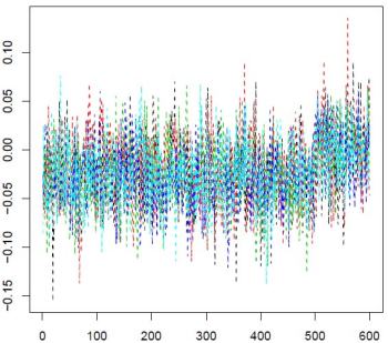
The NAS PC1 is in black. You can see how the other eigenvalues are picking up the variation in the HS shaft, and settling into a Sturm-Liouville pattern.. The decentering concentrated the blade variability in PC1.
Update. This actually shows what decentering is doing. The S-L pattern with orthogonal polynomials, say, start with constant 1. So you would in PCA, if you didn't subtract the mean. It reflects the chief common pattern, which is offset from the mean. 

 But that's not interesting, and subtracting the (centered) mean promotes the second eigenvector to leading. It makes no radical difference, but saves arithmetic.

 Decentered, that constant PC comes back, with a kink. Again, it makes little real difference. You may just have to use one extra PC in the recon.

Reconstruction

In reconstruction, we project the data (matrix X) onto the space spanned by some small number of eigenvectors, and calculate some average. In a real recon, it will probably be some spatially weighted average. The weights are not dependent on the PCA; they represent whatever integral you are trying to reconstruct. Here it might as well be a simple average. If L is the nxp truncated matrix of orthonormal eigenvectors (n=data, p= eivecs), then the projection is simply, fourier-like:
y=L*(t(L)*X)
You can see why the sign of PCs doesn't matter. L is there twice. Then the recon is just the row mean of this matrix.

So I'll calculate the 5 recons of another set of random data using just one PC. I've used the NAS HS index to orient, and scaled by standard deviation of the whole curve. I should say that this is not justified at all in general; while PC's are sign insensitive, recons certainly aren't. However, we're reconstructing essentially zero plus noise. I'll then show what it looks like without scaling.



With one PC and the scaling, it looks HS-like, reflecting the PC itself. Without scaling it looks like this:



This reflects the fact that while the PC maximises the magnitude of the data in the new basis, the scalar product with another vector, which is the recon, can be of different size and sign. In this very simple analogue, we're reconstructing zero plus noise. Anything can happen.

OK, now we try a recon with 2 PC's, rescaling again by HS index etc. Still the same data (for all recons, not re-randomised).



Still a bit of HS, but not much. How about 3:



All gone. And three PC's would be a small number of PCs to retain in a reconstruction.

Remember, this was the extreme case of AR1(0.9), where the HS effect on PC1 was very large. But it was not creating HS effect from nowhere. It was just transferring it from other PCs to PC1.

The code, adapted from the NAS code, is here.

Appendix. 

McIntyre and McKitrick, in their Energy and Environment paper, 2005, showed their emulation of MBH, with and without de-centering. Brandon has alluded to this in comments. I'll show the plot here:

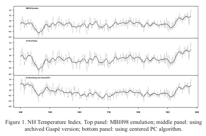
Top is their emulation of MBH, decentered. The bottom figure combines the effect of centering and removal of Gaspe cedars (which I think is unwarranted). It's a pity they didn't show just the effect of decentering, but even so, it isn't much. It shows that PC1 doesn't have much to do with the outcome.

ClimateBall at Climate Audit

There's a post at Climate Audit on Kevin O'Neill's comments exposing aspects of the Wegman report. I would like to respond there, but am currently not able to. All my comments go to spam, and at CA, they don't re-emerge.

I'll say a little about this situation. It affects my interaction with all Wordpress blogs. Last month I was temporarily banned at WUWT, in circumstances I describe here. The mechanism is that I was designated a spammer, and my comments went to spam. After a week or so, I tried commenting again, but same result. This apparently was picked up by Akismet, and my comments at CA started going into moderation, then into spam. Same at other Wordpress blogs.

I can comment using my Twitter ID, but CA does not allow that. WUWT nominally does, but my comment was removed because Twitter substitutes my Twitter address for the email address. So I'm out there too.

Anyway, back to CA. Back in 2010, DeepClimate noted some strange features of the Wegman report. There was much plagiarism, but also the statistics had some very odd features. One concerned the trumpeted claim that Mann's algorithm would create hockey sticks out of red noise input. Wegman showed a dozen profiles generated by red noise. He said in the caption to Fig 4,4:

"One of the most compelling illustrations that McIntyre and McKitrick have produced is created by feeding red noise [AR(1) with parameter = 0.2] into the MBH algorithm. The AR(1) process is a stationary process meaning that it should not exhibit any long-term trend. The MBH98 algorithm found ‘hockey stick’ trend in each of the independent replications."

As DC found, what they had actually done, using M&M's code, was to do 10000 runs with red noise input, select the top 100 by hockey stick index, and then select randomly from that 100. I described the consequences of this here. I showed, inter alia, that selecting that way gave hockey sticks whether you used Mann's off-centre PCA or centered PCA.

Brandon Shollenberger responded by trying to move the goalposts. The selection by HS index used by Wegman had the incidental effect of orienting the profiles. That's how DC noticed it; the profiles, even if Mann's algorithm did what Wegman claimed, should have given up and down shapes. Brandon demanded that I should, having removed the artificial selection, somehow tamper with the results to regenerate the uniformity of sign, even though many had no HS shape to base such a reorientation on. And so we see a pea-moving; it's now supposed to be all about how Wegman shifted the signs. It isn't; its all about how HS's were artificially selected. More recent stuff here.

So now Steve McIntyre at CA is taking the same line. Bloggers are complaining about sign selection: "While I’ve started with O’Neill’s allegation of deception and “real fraud” related to sign selection,...". No, sign selection is the telltale giveaway. The issue is hockey-stick selection. 100 out of 10000, by HS index.

Update. It seems that if I disown my WP id, and change my name slightly, I advance at CA from the spam bin to the moderation queue (probably as a first time commenter). That can be a long wait too, but we'll see.
Update. In comments, Rachel from "Engineering Happiness" made a helpful suggestion about contacting Akismet. I followed advice, and someone emailed me. Not solved yet, but we're working on it. Thanks, Rachel.

Mesh peel

I've long been interested in what can be done with irregular triangular meshes. And lately I've been using them a lot, in apps like this. If you have a set of data on the Earth with no special pattern, like temp measurements, then the best way for both analysis and graphics is to create an irregular mesh of triangles joining the points. Here is an HTML 5 version which allows you to display the mesh.


In earlier times in finite elements, problems on meshes were often solved with direct solvers, which greatly benefit from a banded matrix. This depends on node numbering. On a regular grid, you'd number by rows; in an irregular mesh something of that can be achieved by an advancing front, which passes through every node, and numbering is by order encountered.

I have found two current requirements for a front. One is in a shorter way of defining the mesh, for web transmission. And the other is in WebGL. For the latter, I've developed a more easily visualized method, which, as you might guess, leads to pretty pictures. And yes, WebGL. It describes the mesh as a peel. The rind is one triangle thick - each triangle has two nodes on one side, and one on the other. Well, mostly. Details below.
Update: I found that the original mesh had some incorrectly oriented triangles. The method assumes consistent orientation, so it's rather surprising that the algorithm ran to completion. Anyway, it looks much more regular now.

Mesh specification

You can't avoid listing the lat/lon of the nodes. The simple and usual way of listing the connecting lines is by listing each triangle. But there are typically about twice as many triangles as nodes, so each node gets mentioned six times in total, on average.

If you can reproduce the motion of a moving front, you only specify each node once, when it is encountered. Since the front passes through each triangle, about half the triangles are created without listing a new node (infilling), although a few bits of info are needed to indicate the kind of infill. This is what I currently do, and it is a big plus for the apps mentioned above. But the front does not advance in an easily visualized way, and so for WebGL I need something else.

The WebGL issue

I've described the use of WebGL elsewhere, for example here. Because it's highly parallel, it tends to be very verbose, since it sends copies of everything rather than use pointers. So every time you mention a node, it is by coords and color - 7 floats. And as above, the default spec by triangles mentions each node about six times.

WebGL mitigates this with two structures - TRIANGLE_FAN and TRIANGLE_STRIP. The first is just a ring of triangles around a node. The second is a strip of rectangles with diagonals (all the same way). The saving is that in each, nodes are mentioned once, in each strip, say. That's twice in total, instead of six.

The strip sounds a bit limiting, but there are various ways you can stop and start. You can add degenerate triangles.

So my ambition here is to develop a front that works like peeling an orange with one continuous rind. I don't have the strip in WebGL working yet. But I do have pictures.

The algorithm (briefly)

It works by in effect rolling a triangle from start to finish. Not the same triangle, but moving from one to another in a series of fans. I rotate anticlockwise. There is always a front dividing "old" and "new", and when the fan reaches "old", it switches pivots, and starts another fan.

The picture below shows this with shading. The "old" side of the peel is blue, the new is red. There is a blue line joining the centroids of the triangle in number order. Sometimes the rolling gets stuck; it tries a new pivot, but can't move. You'll see those as solid blue triangles in the pic. It escapes by backtracking to the nearest pivot that can move. It's also possible that the front can form a pocket, leaving behind a set of triangles. There's provision for it to check and go back and fill in those areas. There will be a cost in describing that, but it doesn't happen often.

The result

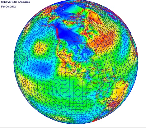
So here is a picture of about 4000 stations (GHCN/ERSST) that reported in some recent month (I've lost track of which). The mesh comes from R's convhull(). There is a red triangle in the Mediterranean where it starts, and end in a white triangle in the W Pacific. I think it is quite interesting how it adapts to very different density in, say, US vs Africa or Antarctic. It's like a big spiral, and as mentioned above, the "old", or inside edge is blue, outer red. The usual WebGL facilities - Earth is a trackball - right button drag up or down to zoom.