But still it's an interesting analytic problem, so I did some analysis. It particularly concerns the role of persistence, or autocorrelation. Increased autocorrelation tends to show more effect, because for a given number of proxies, it diminishes the effect of noise relative to the underlying short-centering operator (graphs below). But that underlying pattern is interesting, because it is much less dependent on autocorrelation. And the next PC's in succession are interesting, as I wrote about here.
White noise
You need an infinite quantity of proxies to see a pattern with white noise. But the pattern is the prototype for more difficult cases, so I'll develop it first. Much of what I have done recently is based on the work in the NAS report and its associated code. They compute and scale not only PCA first components from AR1() proxies, but also from the associated correlation matrices, which they scale and put on the same graph.
The algebra of short-centered averaging works like this. Define a N-vector h which has zeroes outside the short averaging period (M years at the end of N years of data), and values 1/M within, and another vector l which has 1's only. Then for a data vector x, length N, the valkue with short mean deducted is x-l*(h.x), or E*x, where E=I-l⊗h. I is the identity matrix, and ⊗ the dyadic product. For future reference, I'll note the dot products
l.l = N, l.h = 1, h.h = 1/M.
Then for a data vector X, Nxp, p the number of proxies, the PC's are the eigenvectors of XX*. The expected value of this, as a random noise vector, is p*K, where K is the autocorrelation matrix. For eigenvectors we can drop the p. The short-averaged version is E*X*X**E*. So for white noise, K is the identity I, and we need just the eigenvectors of E*E*.
Expanding, the eigenvalue equation is
(I-l⊗h - l⊗h + l⊗l h.h)*u = z u
or
(l⊗h + l⊗h - l⊗l h.h) u = (z-1) u
Since the matrix on the left now has range spanned by l and h, u must be in this space too. So we can set u = A*h+B*k, and there is a 2-dim eigenvalue for u in this space. I'll skip the 2-d algebra (just substitute u and work out the dot products), but the end results are two eigenvalues:
z=0, u=l
z=N/m, u= l-h
The latter is clearly the largest eigenvalue. There are also a set of trivial eigenvalues z-1=0; these correspond to the remaining unchanged eigenvalues of I.
So what has happened here? The short averaging has perturbed the correlation matrix. It has identified the vector u=l-h, which is 1 for years in 1:(N-M) and zero beyond, as the first principal component. This will appear in any reduced set of eigenvalues. All vectors orthogonal to it and l are still eigenvectors. So no new eigenvectors were created; u had been an eigenvalue previously. It just means that now whenever a subset is formed, it will come from a subset of the unperturbed set. They were valid bases for the space before; they still are.
Effect of autocorrelation.
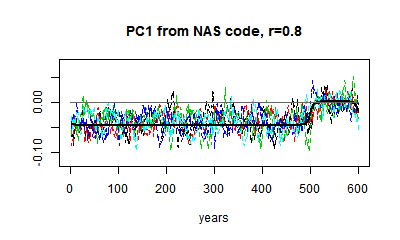
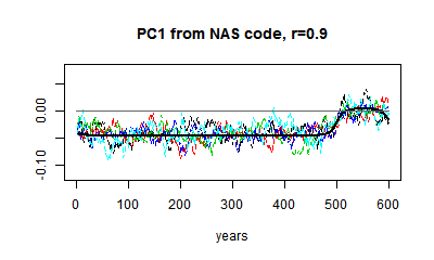
I showed earlier DeepClimate's rendering of two AR1() cases from the NAS code: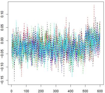 |  |
| AR(r=0.2), 5 PC1s from sets of 50 proxies. | AR(r=0.9) |
You can see that relative to the HS effect, the noise is much greater when r=0.2 (it depends on proxy numbers). And I can't usefully show white noise, because the noise obliterates the effect. but the eigenvector is not very different.
Here are some plots of PC1 from r=0.1 to r=0.9. I've kept to the same scale. You can see the gradual change in the matrix eigenvector, and the gradual downscaling of the noise, which makes the eigenvalue pattern stand out more.
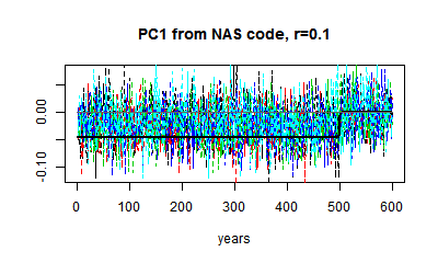 | 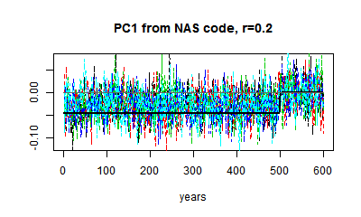 |
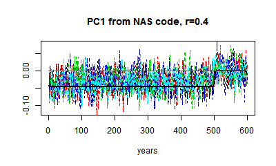 |  |
 |  |


Playing with your code ...
ReplyDeletehttps://github.com/rbroberg/rhinohide.org/blob/master/climate/other_peoples_code/stokes/recon2014/Moyhurecon-revised.r
The Wegman Report already did a mathematical calculation of the bias in the eigenvalue.
ReplyDeleteWhere do you think they did a bias analysis for the actual data?
DeleteAs opposed to standard math and general description of how to do it? (Appendix A)
Have you checked it for plagiarism?
DeleteJean S also has a discussion here .
ReplyDeleteNick,
ReplyDeleteI noticed this post only after writing my previous comments. They might have suited also in this thread.
I think that you made some errors in your mathematics. The covariance matrix, whose eigenvalues and eigenvectors are determined is not XX*, but X*X in case of time series that have already been centered. The difference is essential.
Carrick linked to a comment of Jean S and Steve added there a further link to Wegman report. The Appendix A of Wegman report seems to contain in A.3 a correct description partly in component form. I may add soon a similar description using fully matrix notation. I that connection I may add some further comments on what that means for the results.
Pekka,
Delete"The covariance matrix, whose eigenvalues and eigenvectors are determined is not XX*, but X*X in case of time series that have already been centered. The difference is essential."
Pekka,
The non-zero eigenvalues are the same:
Proof if X*Xu=λu, then (XX*)Xu=λ Xu,
This is behind the svd decomposition.
Here I need to look at XX*, because I am applying the short-centering operator. The eigenvectors I want are time series.
Nick
DeleteIn the correct mathematics the factors from short-centering ends up between X* and X, not outside as in your derivation.
A preliminary version of my derivation is here: http://pirila.fi/energy/kuvat/PCAComments.pdf
Pekka,
DeleteI am following the logic of the NAS progran cited earlier. By svd, X=UdV, where U is the set of nontrivial eigenvectors of XX*, V the eivecs of X*X and d the set of common eigenvalues. The first column of U is the PC1 that we know and love. I am looking at the effect of short centering (operator S) on PC1, so it is that U analysis that I need. I am looking for the first eivec of SXX*S*. S operates on the columns of X.
The eigenvectors of this modified matrix are still orthogonal (symmetric). They are not orthogonal with the kernel XX*.
I read your analysis, but I don't see how it can yield a time series PC1. It's the analysis of V, not U.
Nick,
DeleteIf I understood you correctly, we have in my notation
U = YV = BXV
Pekka,
DeleteYes. SVD gives U, which are the PC's as time series, and V, which are the coefficients which combine the columns of X to produce those series. U are the non-trivial eigenvecs of XX*; V eivecs of X*X. As you say, they are closely related, and you can do an eival analysis of X*X, as you do, to get the coefs, and then combine, or do a direct eival analysis of XX*, as I do.
Nick,
ReplyDeleteI had perhaps too strongly in mind, how the short-centered analysis proceeds in practice rather than the task of figuring out consequences of assuming specific noise models and applying short-centering.
Mentioning the words "non-trivial" in the original post might have been helpful in leading thoughts to the right track.