Tails of the Pause.

I've been writing lately about matters which, I'm sorry to say, lack scientific gravity. One is the possible record warm 2014, and the other is the tailing of the Pause, as measured by periods of negative trend. My excuse is, people do talk about them, and there is interesting arithmetic which I can illustrate.

In my "pause" posts, I showed plots of trend of global temperature to present, plotted for periods shown on the x-axis, with trend shown at the starting point. A "pause" starts when, for some index, the axis is first crossed from pos to neg. The plots were active, and you could see the curves rising steadily over recent months. This meant the start of the pause moves forward, with eventual jumps where a previous excursion below the line no longer makes it.

Here is the recent active (buttons) plot to show that effect:


In this post, I'll quantify the rate of motion, and describe how much cooling would be required to reverse the trend. The effect of a new month's reading depends on its status as a residual relative to the regression line for the period - ie is it above or below the line, and by how much. But one reading is a different residual for each such period. I plot the present month as a residual, again referred to the start year, and also plot the rate of change of trend produced by the current (August) temperatures.

Rate of change

This is more simply described with a continuum version. A time period runs from 0 to x, with readings y. If x increases, what is the change to trend β. The continuum formula is β = (x ∫ xy dx - x*x/2 ∫ y dx)/(x^4/12)
Note that y occurs only in integrals (which are from 0 to x), so when we differentiate β, no need to differentiate y. So, after some calculus algebra,
dβ/dx = (6/x^2)(y - y0 - βx/2)
where y0 is the mean over the period. Since the regression passes through this mean midway, the last part of this is the end residual.
ie dβ/dx = (6/x^2) * residual
That gives the factor that determines the rate.

So my first plot is the rate of rise, shown as a 3 month incrementwith August trends dotted



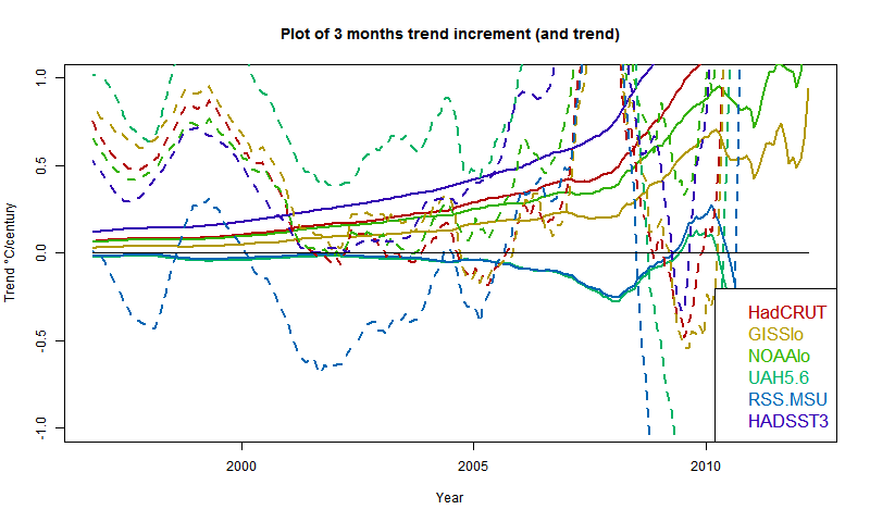
The satellite measures aren't going to move much without substantial warming. However, UAH is already high, RSS is low. Of the surface indices, HADSST3 is rising fast, GISS relatively slowly. However, three months of current warmth makes a big difference to the pause.

And here is the plot of residuals of August temp relative to past regressions:



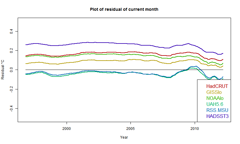
It confirms that UAH and RSS are near zero, so continuation of present temps won't change anything (though UAH warmed in Sept). Otherwise, GISS has the lowest residual, but positive everywhere; HADSST3 the highest. This of course partly reflects past coolness of HADSST3.

So if temperatures drop about 0.07°C from August, the rise for GISS would pause (but GISS rose in September). It would take a drop of more than 0.2°C for HADSST3.