Recent interest in PCA and paleo has got me doing some stuff I should have done a while ago. I think it is bad that Steve McIntyre and Wegman have been able to maintain focus on just the first component PC1, leading people to think they are talking about reconstructions. They aren't, and that's why, whenever someone actually looks, the tendency of Mann's decentered PCA to make PC1 the repository of HS-like behaviour has little effect on recons. I'll show why.
Steve's post showed Fig 9.2 from the NAS report as an example of an upright PC1. That's got me playing with the NAS code that generated it. It's an elegant code, and easily adapted to show more eigenvalues, and do a reconstruction. So I did.
Mann pointed out many years ago that M&M had used too few PC's in their recon. Tamino explained that PCA simply created a different basis, aligned to some extent with real effects, which may be physical. But there is conservation involved - if HS behaviour is collected in PC1, then it is depleted in PC2,3 etc, and in the recon, it averages out.
And it does. For the NAS example, I'll show how the other PC's do have complementary behaviour, and since the HS effect of decentering isn't real physical, but drawn from other PCs, it doesn't last when you use more PCs, as they do.
The NAS, I should note, did not intend their simple example to have real tree-like properties. They chose a AR1 model of extremely high persistence (r=0.9) - decadal weather - to emphasise the effect of decentering. Wegman said that his Fig 4.4 was based on AR1(r=0.2), which may be more realistic, but wasn't what the code did. Anyway, DeepClimate showed the two plots thus (x axis in years):
 |  | |
| 5 PC1s generated from AR1(.9) (left) and AR1 (.2) (right) red noise null proxies. | ||
Each curve is the result of decentered PCA (last 100 years) on a set of 50 AR1(r) 'data'. Obviously, the r=0.2 version is much less HS-like, but still some. One of the elegant features of the NAS code is that they calculate the theoretical PC for the model, which is just the first eigenvalue of the autocorrelation matrix. I have some analytic theory here, for a coming post, but I'll just say for now that the HS-ness is about the same for low values of r; for 0.2 it is just beginning to increase.
I'll look at the decentered r=0.9 case for emphasis, and as an extreme worst case. The theoretical eigenvalues from the autocorrelation, calculated NAS-wise, look like this:

The NAS PC1 is in black. You can see how the other eigenvalues are picking up the variation in the HS shaft, and settling into a Sturm-Liouville pattern.. The decentering concentrated the blade variability in PC1.
Update. This actually shows what decentering is doing. The S-L pattern with orthogonal polynomials, say, start with constant 1. So you would in PCA, if you didn't subtract the mean. It reflects the chief common pattern, which is offset from the mean.
But that's not interesting, and subtracting the (centered) mean promotes the second eigenvector to leading. It makes no radical difference, but saves arithmetic.
Decentered, that constant PC comes back, with a kink. Again, it makes little real difference. You may just have to use one extra PC in the recon.
Reconstruction
In reconstruction, we project the data (matrix X) onto the space spanned by some small number of eigenvectors, and calculate some average. In a real recon, it will probably be some spatially weighted average. The weights are not dependent on the PCA; they represent whatever integral you are trying to reconstruct. Here it might as well be a simple average. If L is the nxp truncated matrix of orthonormal eigenvectors (n=data, p= eivecs), then the projection is simply, fourier-like:y=L*(t(L)*X)
You can see why the sign of PCs doesn't matter. L is there twice. Then the recon is just the row mean of this matrix.
So I'll calculate the 5 recons of another set of random data using just one PC. I've used the NAS HS index to orient, and scaled by standard deviation of the whole curve. I should say that this is not justified at all in general; while PC's are sign insensitive, recons certainly aren't. However, we're reconstructing essentially zero plus noise. I'll then show what it looks like without scaling.

With one PC and the scaling, it looks HS-like, reflecting the PC itself. Without scaling it looks like this:

This reflects the fact that while the PC maximises the magnitude of the data in the new basis, the scalar product with another vector, which is the recon, can be of different size and sign. In this very simple analogue, we're reconstructing zero plus noise. Anything can happen.
OK, now we try a recon with 2 PC's, rescaling again by HS index etc. Still the same data (for all recons, not re-randomised).

Still a bit of HS, but not much. How about 3:

All gone. And three PC's would be a small number of PCs to retain in a reconstruction.
Remember, this was the extreme case of AR1(0.9), where the HS effect on PC1 was very large. But it was not creating HS effect from nowhere. It was just transferring it from other PCs to PC1.
The code, adapted from the NAS code, is here.
Appendix.
McIntyre and McKitrick, in their Energy and Environment paper, 2005, showed their emulation of MBH, with and without de-centering. Brandon has alluded to this in comments. I'll show the plot here: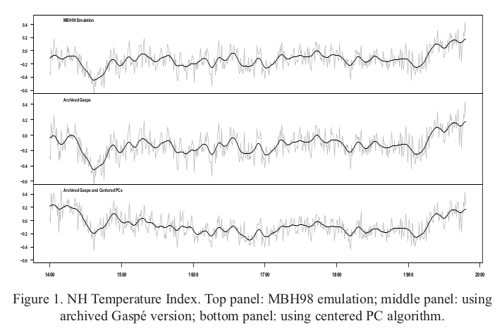
Top is their emulation of MBH, decentered. The bottom figure combines the effect of centering and removal of Gaspe cedars (which I think is unwarranted). It's a pity they didn't show just the effect of decentering, but even so, it isn't much. It shows that PC1 doesn't have much to do with the outcome.


I struggle to remember this stuff, but:
ReplyDelete> the other eigenvalues are picking up the variation in the HS shaft, and settling into a Sturm-Liouville pattern
Doesn't that mean you're seeing what often happens with lower EOFs, which is there's no real physical structure in there. Its just noise. You're seeing (apart from the leading EOF, and required orthogonality to that, and perhaps for the "blade" bit) what you'd see from any old random noise?
The Sturm-Liouville comes from the autocorrelation. If you have AR1(), centered, then the inverse of the autocorrelation is basically tridiagonal, and has the same eigenvectors. A second order recurrence with a linear parameter - classic S-L. The decentering perturbs it a bit, as does the Hosking structure used by M&M, but that's how the higher eivecs work. And yes, all that comes from noise, but reflects its structure. That's all there is in this example. But it does show how the decentering effect fades when you reconstruct properly.
DeleteVery interesting post, Nick. While I"d say you're "moving the goal posts" here, you're moving them towards practical questions. So progress.
ReplyDeleteCan you think of a way to test whether there is an effect on the signal to noise in the reconstruction from the non-centered PCA?
I can imagine this might be an issue for systems with very poor SNRs.
I'm traveling now so I'll post infrequently, but will read with interesting any comments you make.
Carrick,
DeleteWell, here there is no signal. But I could add one. I'll check if it helps.
Thanks Nick. Ultimately the real question is in understanding the impact of short-centering on Mann's algorithm, which is why I was nudging you on the issue of thinking about what happens to signals (effect on SNR and also on bias of course).
DeleteNick,
ReplyDeleteReconstructions have a temperature history target (eg instrumental temperature record). What is the target for your reconstruction with synthetic data?
Steve Fitzpatrick
Steve,
DeleteThere's no target here. The signal is zero. I'm (like NAS) just looking at the effect of AR1 noise and decentering. There wouldn't be any point in trying to line up these "proxies" with a target, because we know they are random.
Nick,
ReplyDeleteI think lining them up with a specific target series is THE key issue here. A reconstruction based on pink noise synthetic data series and a "flat" target (AKA no signal) will of course generate a flat reconstruction (how could it do otherwise?). Reconstructing based on a rising target near the end of the reconstruction period (as is actually done with real data) seems to me the only meaningful test of bias in the reconstruction method. I am not absolutely certain, but I strongly suspect that if you reconstruct a large collection of synthetic pink (eg r=0.2 or 0.3) noise series (say 100) this way, you will find that they do consistently generate artificial hockey stick reconstructions if the target is a sharp rise near the end of the period. What I am saying is that the automatic adjustment in the sign of the correlation, combined with weighting to optimize the match with the target, guarantees the reconstruction will mimic the target, whatever that target shape is. (I am for sure not the first person to suggest this!)
Steve Fitzpatrick
Steve,
DeleteWhat I'm trying to show with this simple example is how PCA is followed by operations in which some aggregate is formed by mapping onto the lower dimensional space and then combining in some way. I agree that Mann's process, say, has more complex steps. I'm pushing back against the idea that a shape distortion in PC1 can be identified with a shape distortion in the result.
"What I am saying is that the automatic adjustment in the sign of the correlation, combined with weighting to optimize the match with the target, guarantees the reconstruction will mimic the target, whatever that target shape is."
I'm not sure what you mean by the adjustment of the sign. But yes, the process is designed to push the recon to match the target. That is an argument for discounting the apparent appearance of 20thCen rise (or decline) in the result. The proxy process is designed to align with the recent to learn about the past. To actually know about the recent, we have thermometers.
Nick,
Delete"That is an argument for discounting the apparent appearance of 20thCen rise (or decline) in the result."
No, I think it is more an argument for questioning what in the proxy series data causes the reconstruction to fit the target series, and so an argument for questioning the accuracy of the reconstruction *before* the target period. Is the match with the target series due to a real signal, or is it just a manifestation of pink noise... or some of both. If pink noise series (of some reasonable redness level), where we know there is zero real 'proxy information', can produce a match to the target series in the reconstruction, then it seems to me the method is clearly biased toward producing a reconstruction which matches the target series, even when we know the entire "reconstruction" comes from nothing but pink noise, and so is rubbish.
Now, there very well could be some real climate signal mixed in with pink noise in real proxy series, but It seems to me you have to account for how much pink noise in the real proxy series can contribute to the fit with the target series to have any confidence in the accuracy of the reconstruction before the target series.
Steve Fitzpatrick
Nick, If you are interested in Sturm-Liouville formulations, again consider following the work at the El Nino project. I am contributing a Mathieu differential equation formulation, which has some promise as an exploratory and potentially predictive model.
ReplyDelete.
Thanks WEB. Yes I did read that. Couldn't think of anything to contribute at the time, but I'll re-read. I did contribute to the thermo thread. The tidal stuff seems to be making progress.
DeleteThe Sturm-Liouville class of behaviors includes the Mathieu formulation as a variant. These all share the same characteristic of being a form of second-order differential equation distinguished by how the potential well is shaped, thus leading to different oscillating responses. The model of red noise definitely fits into this category as a stochastic variant, as the red noise drag factor defines how steep the well is; so when the random walker tries to climb out of the well it will have a bias to revert to the mean. Of course this works in both directions, so the response is symmetric.
ReplyDeleteNick,
ReplyDeleteMaybe you can clarify something for me. As I understand it, by using AR1(0.9) they were producing random datasets that actually had hockey stick-like features in them because of the persistence. Is this right? So, there is an issue with de-centered versus centered, but at the end of the day, the method will only produce a hockey-stick if there is such a feature in the data being analysed (whether that data is randomly generated or not). If so, the physically motivated question then becomes whether or not such a feature could be climatic in the absence of some kind of change in external forcing (anthropogenic for example). Given that I think the answer to this is, generally speaking, no, that would seem to indicate that discovering such a feature is indicative of some kind of change in external forcing which, for the 20th century, is largely anthropogenic. Is that a fair assessment or am I missing something?
ATTP,
DeleteIn these examples, HS behaviour is produced randomly, and PCA moves the basis vectors so that PC1 aligns with that behaviour. SM calls this mining for hockey sticks, but it's just pointing to them. When PC1 aligns, PC2 and PC3 etc become orthogonal, which is the conservation I talked about.
So yes, you do need HS behaviour to align with; PC1 acts as a concentrator. My point here is that the expression of an average in the PC frame, which is part of a recon, quickly undoes that artificial concentration. Both centered and decentered will reflect in the average the amount of real HS in the sample. PCA can't tell whether it is anthro.
My view is that one shouldn't really look to proxies for answers about recent warming. The analysis process selects for alignment with instrumental, so it doesn't really confirm it independently. Instrumental is much better anyway, so we don't need the confirmation.
Nick, thanks. Yes, I agree that PCA can't tell if it's anthro, but it does tell us that it exists. Also, I agree with your latter point completely. The more interesting aspect of these paleo reconstructions is what they say about the era prior to when anthropogenic forcings started to increase. They appear to indicate that our climate has been broadly stable for at least 1000 years and, given Marcott et al., possible for most of the Holocene. I was really just trying to understand the significance of the AR1(0.9) choice, and I think I now do.
DeleteNick, do you have an opinion on why some are so hesitant to admit that the AR1 lag coefficient used to generate the PC1 'hockey stick' was ≈ .9? Consider the following exchange with Brandon Shollenberger, this is not the first time I've run into this resistance - just the most recent.
ReplyDelete-----------------
KTO: "Brandon, as the NRC/NAS study showed, they had to use AR1(.9) to achieve the result M&M got with their ‘persistent red noise’ model or that Wegman got with his AR1(.2). So we’re comparing AR1(.2) to AR1(.9) The implied persistence is 1.5 years versus 19 years."
Brandon: "This is complete BS as anyone who reads our conversation knows. Leaving aside the fact you are simply making things up when you say": (kto)"the NRC/NAS study showed, they had to use AR1(.9) to achieve the result M&M got"
-------------------
I've provided Brandon with the following references
” Figure 9-2 shows the result of a simple simulation along the lines of McIntyre and McKitrick (2003) (the computer code appears in Appendix B).”
NAS Report Page 90
http://www.nap.edu/openbook.php?record_id=11676&page=90
phi <- 0.9;
NAS Report Appendix Page 140
http://www.nap.edu/openbook.php?record_id=11676&page=140#p200108c09970140001
Kevin,
DeleteMy interpretation is that the NAS just chose a number that was adequate for that purpose, which was to create a highly visible effect. I didn't take it that they were trying to quantitatively match M&M; and I think theirs is a bit more exaggerated.
The M&M method is rather hard to analyse (and takes an awfully long time to run). There is a different persistence for each proxy. It would be hard to match with ARx().
[previous comment continued]
DeleteIn that RC article, von Storch is roundly criticised for using a co-efficient of .7, which as Ritson says:
"Von Storch et al added proxy-specific noise that was highly correlated from year to year. It was characterized as AR1, or a simple Markoff process, noise with 70% of a previous years history carried over from a previous year to the next year (this a corresponds to a one year autocorrelation coefficient of 0.7). A factor of 0.7 corresponds to a decorrelation time of (1+.7)/(1-.7) or 6.3 years and reduces the effective number of independent data-points by the same factor i.e. 6.3. If the noise component of real proxy data were really so strongly red, not only the precision of results of Mann et al. (the target of the von Storch et al's analysis) but indeed of all previous millennial paleo-reconstructions would be substantially degraded."
Well, McIntyre even upped the ante on that score. Instead of AR1(), he used ARFIMA to generate the noise simulations. From the R code in the SI ('2004GL021750-script.final.txt'):
"##2. SIMULATION FUNCTION
#two alternative methods provided: arima and arfima; only arfima used in simulations here"
As Nick and Kevin (and Deep Climate before them) say above, the NAS had to turn the dial all the way up to AR1(.9) before they could get any PCs that looked like the ones McI had extracted from the noise simulations generated using ARFIMA. What's the average de-correlation period of that, then:
(1 + .9)/(1 - .9) = 19 years
According to someone who actually has a clue about this, like Ritson, what McIntyre did so degraded the signal as to render any PCA analysis that was done on it meaningless. So in addition to the 1:100 cherry pick, we also have a noise model that *has no basis in nature*, with way over-cooked persistence. Looks like McI completely botched the analysis in MM05. Was it incompetence or malice? I'd say a bit of both. Obviously, this is not my original work, and all credit must go to Deep Climate for peering into the dark corners where McI doesn't want anyone to look. I'm just 'splainin' it here for the benefit of those who don't want to have it explained to them. So, a final question then: if Carrick *isn't* a McIntyre sycophant as I (rather boldly, I admit) stated in the previous thread, and is supposedly so objectively critical of the man, than how come he doesn't pick up on in-your-face obvious blunders like this, and the disingenuous 1:100 cherry-pick? Hmm.
"the NAS had to turn the dial all the way up to AR1(.9) before they could get any PCs that looked like the ones McI had extracted from the noise simulations generated using ARFIMA"
DeleteThe NAS didn't know (no-one did) about the 100-1 selection. Without that, I think the Wegman style PCs profiles actually do reasonably match an AR(0.2) or so. And as I said above, I wouldn't read too much into the NAS choice. They were saying that the effect was not intuitive, and they wanted to convince people that it was real.
"But how can you generate "trendless" red noise from data that has climate signal in it?"
The hosking.sim package is something of a black box. I've searched for discussion of its use, but found almost nothing. It seems to produce arfima simulations which match the autocorrelation structure of the proxies. To what extent that would transfer signal (HS say), I just don't know. I think it is an unwise choice, but as with decentering, it may not have much negative effect.
"how come he doesn't pick up on in-your-face obvious blunders like this, and the disingenuous 1:100 cherry-pick?"
I think there has been a tribal response. I have wondered what would be said if Mann had made an undisclosed 100-1 selection based on results before presenting those results as representative.
Nick, hi,
DeleteYou said above:
The hosking.sim package is something of a black box. I've searched for discussion of its use, but found almost nothing. It seems to produce arfima simulations which match the autocorrelation structure of the proxies. To what extent that would transfer signal (HS say), I just don't know. I think it is an unwise choice, but as with decentering, it may not have much negative effect.
Steve McIntyre has been harping on for years about how Mann's PCA produces hockey sticks out of nothing, i.e. from so-called "persistent trendless red noise" (my emphasis. But see McI quote down below, for instance). So my point is, quite simply:
a. Either the noise is supposed to be trendless, in which case don't you need to de-trend those 70 tree ring series that have climate signal in them first, before you use them to generate the red noise? Then you shouldn't get any hockey sticks. If we do after that, then there's a problem alright.
or
b. Use them as they are, only inject a *realistic* bit of noise into them to simulate non-climatic effects on the trees like disease or insect infestation. Then we *should* get hockey sticks, if the PCA method used is robust, and can still pick the signal out of noisy proxies.
AFAICT, SM did neither of the above. We only have his word for it that hosking.sim package didn't transfer a non-negligible amount of climate signal to the noise simulations. In fact, it would be very interesting indeed (you know, just for the lolz) to see some plots of a random selection of those noise runs.
Nick,
DeleteThe hosking.sim package is something of a black box.
Interesting that you've said this. I thought it was just me. I tried to do the same and all I found was some old paper that I couldn't really face wading through. What struck me was that I would typically expect people to either use some package that is well understand in the community, or write a routine themselves that they explain properly in their paper. Using a package that appears not to be well documented and that is discussed in only a few lines in the paper is a little bit unfortunate.
When I first started blogging about the whole climate change issue, one of my early posts was about this topic. I understand it better now, but I've always found it a little strange that the trendless red noise in MM05 was generated using the data from MBH98.
Metzo,
Delete"In fact, it would be very interesting indeed (you know, just for the lolz) to see some plots of a random selection of those noise runs."
I could show that. But pretty much equivalent is the set of PC1's shown here, calculated with centered mean and no selection. That should show a pattern if it is coming in through the noise model. There may be some, but it isn't obvious.
ATTP,
AS you probably saw, the main thing that shows up on Google searches is Eugene Wahl in 2006 asking if anyone knows anything about hosking.sim. I presume while he was writing his paper on M&M etc. I don't think he got a response.
Nick, hi again,
DeleteJust an interested layperson, so not spending *too* much time on this (heh). I had to go read MM05 once more, because it was a while back that I first read it and I had to check their methodology again. The start of section 2 reads:
2. Monte Carlo Simulations of Hockey Sticks on Trendless Persistent Series
[6] We generated the red noise network for Monte Carlo simulations as follows. We downloaded and collated the NOAMER tree ring site chronologies used by MBH98 from M. Mann’s FTP site and selected the 70 sites used in the AD1400 step. We calculated autocorrelation functions for all 70 series for the 1400–1980 period. For each simulation, we applied the algorithm hosking.sim from the waveslimpackage version 1.3 downloaded from www.cran.r-project. org/doc/packages/waveslim.pdf [Gencay et al., 2001], which applied a method due to Hosking [1984] to simulate trendless red noise based on the complete auto-correlation function.
So they captured the auto-correlation function for each of the 70 tree ring series, and then generated red noise based on the auto-correlation functions. The hosking.sim package uses ARFIMA, which has a long memory (hyperbolic decay) as opposed to something like AR1(.2) which is what Wegman assumed McI used. Now... assuming that none of the climate signal that was in the non-detrended proxies carried over into the output, there is still a concern I have (I guess I'm concern trolling now, but this *is* Climateball™ we're playing, m'kay? :-). And that is:
If the year-to-year auto-correlation of the proxies is weaker along the shaft of the hockey stick when the climate is relatively stable (a very slow down-trend heading toward the next glaciation period), and gets stronger during the 1902 - 1980 calibration period (the blade of the hockey stick when we start to see the marked effects of, you know, global warming)... then that would cause a certain amount of the noise simulations to 'run away' at the very end because of the extra-long persistence of the ARFIMA-based noise. This, of course, makes the noise look just like a global warming (or cooling, if it goes negative!) signal.
If my assumption is incorrect that the auto-correlation function for each proxy time series behaves differently during a period of relative stability then it does during a period of fairly rapid change, then please feel free to correct me (as if the folks here would be shy about that :-) This comes back to my point about whether or not the noise model used in MM05 is appropriate or not. I'm thinking not.
This comment has been removed by the author.
DeleteSteve McIntyre and Ross McKitrick have never disputed a hockey stick can be found in the data. Their published work specifically says if you implement PCA properly, you get a hockey stick as NOAMER PC4. If you keep four PCs for the NOAMER network instead of the two MBH kept, you do get a hockey stick. This point has been well established for nearly a decade.
ReplyDeleteAs such, when you say:
I think it is bad that Steve McIntyre and Wegman have been able to maintain focus on just the first component PC1, leading people to think they are talking about reconstructions. They aren't, and that's why, whenever someone actually looks, the tendency of Mann's decentered PCA to make PC1 the repository of HS-like behaviour has little effect on recons. I'll show why.
You are guilty of what you accuse others of. Nearly ten years ago, McIntyre clearly laid out the effect of MBH's de-centered PCA, explained what effects it had on the final results and showed what results one could get when using several alternatives. You haven't done anything like that. You haven't even attempted to discuss the effect various things would have on MBH's results. You haven't even discussed what other data was used by MBH. It's easy to do, so I will. Here is a post where I showed all the proxies used by MBH in their 1400 step:
http://hiizuru.wordpress.com/2014/02/18/manns-screw-up-3-statistics-is-scary/
It shows there were two proxies with a hockey stick shape. One was what is commonly known as the Gaspe series. MBH used it two times. One of those times, it was included in the NOAMER network from which the famous PC1 is calculated. The other time, it was used on its own as a standalone proxy. That time, it was artificially extended so it could be used in the 1400 step. None of this was disclosed by MBH, much less explained (Further discussion and references here). The other was NOAMER PC1.
As long as you include either of those proxies, MBH's methodology will produce a hockey stick. The other 20 proxies used along with them are practically irrelevant. If MBH had implemented it's PCA properly and included only the first two PCs, it would still have gotten a hockey stick because of the (inexplicably duplicated and extended) Gaspe series. If they had implemented PCA properly and removed the Gaspe series, they could have still gotten a hockey stick by including the first four NOAMER PCs.
All of that was established a deacde ago. In the end, the discussion comes back to the 22 series I plotted in the post linked to above. Maybe you think a single tree ring series can be copied out of the NOAMER network, artificially extended so it meets an inclusion criteria then used on its own. Maybe you think we should include as many PCs as we need for the NOAMER network to produce a hockey stick. I don't think either position is justifiable, but whatever. At best, you can come up with two proxies that have a hockey stick shape. Two out of 20+ is ~5%.
MBH rescales proxies by their correlation to the temperature record. That means as long as a single proxy has a hockey stick shape, MBH's methodology will produce a hockey stick. It doesn't matter if that hockey stick come from 5% or less of their data. People focus a lot on the PCA step, but the reality is MBH's rescaling by correlation is even more biased. It's like the screening fallacy on steroids.
"McIntyre clearly laid out the effect of MBH's de-centered PCA, explained what effects it had on the final results and showed what results one could get when using several alternatives."
DeleteHe certainly didn't do it clearly. When Wegman was asked by Rep. Stupak:
"Does your report include a recalculation of the MBH98 and MBH99 results using the CFR methodology and all the proxies used in MBH98 and MBH99, but properly centering the data? If not, why doesn’t it?"
he responded:
"Ans: Our report does not include the recalculation of MBH98 and MBH99. We were not asked nor were we funded to do this. We did not need to do a recalculation to observe that the basic CFR methodology was flawed. We demonstrated this mathematically in Appendix A of the Wegman et al. Report. The duplication of several years of funded research of several paleoclimate scientists by several statisticians doing pro bono work for Congress is not a reasonable task to ask of us. "
Not once, in either the report or when put on the spot in the Committee, did he refer to "McIntyre clearly laid out the effect of MBH's de-centered PCA". There was some belated discussion of Wahl and Ammann.
In fact MM05EE only showed the result after also removing the Gaspe cedars. Even then, the difference is small. That, I think, is why it was little publicized, so even Wegman didn't refer to it.
Nick Stokes, I'm happy to discuss the minor point of whether or not what I explained was clearly laid out nearly ten years ago but only if we also discuss what I explained. There's no point discussing how old the points I've made are if you're going to refuse to discuss the points themselves.
DeleteUntil then, I'll point out it seems strange to say:
In fact MM05EE only showed the result after also removing the Gaspe cedars.
In reference to a graph which showed the effect of removing Gaspe then the effect of removing Gaspe + NOAMER PC1 when the text says when removing the NOAMER PC1:
MBH-type results occur only if a duplicate version of the Gaspé series is used as an individual proxy and the portion of the site chronology with 1–2 trees is used and if the first four years of the chronology are extrapolated under an ad hoc procedure not otherwise used in MBH98.
Given MM05EE made it clear you have to remove both the Gaspe and NOAMER hockey sticks, there would have been little reason to show the removal of just the NOAMER one in the graph you refer to. It would have been highly similar to the one showing the effect of removing just Gaspe. Given the limitations on space, there's little reason to expect people to show such an uninformative result which was specifically discussed in the text.
Side note, I don't think many people will agree with you when you claim the effect shown in MM05EE was small. One is a hockey stick. The other is not. Michael Mann became famous because of his reconstruction being a hockey stick. That wouldn't have happened if his hockey stick stopped looking like a hockey stick ~halfway through (1400 in a 1400-1980 reconstruction).
Brandon,
Delete"Side note, I don't think many people will agree with you when you claim the effect shown in MM05EE was small. One is a hockey stick. The other is not. "
Are we talking about the same thing here? I'm referring to Fig 1 in MM05EE. I've added an appendix to show this plot. I don't think your characterisation is right.
Nick Stokes, again, I can't help but notice you choose to ignore the majority of my comment. If you don't want to discuss most points, nobody can make you, but it is pretty silly to have a section for comments if you'll just ignore most of what commenters say.
DeleteIn any event, yes, we are talking about the same figure. The bottom panel is clearly not a hockey stick. It shows 1400 AD temperatures as higher than 1980 AD temperatures, a direct contradiction of multiple claims in MBH98. And that figure only shows what happens to period covered by MBH98. It's an even bigger problem if the results are extended back to 1000 AD to compare to the full MBH reconstruction. Nobody would have thought it a hockey stick if the middle of the "shaft" was higher than the highest point of the blade.
Forgot to add that Brandon's claim starting with "Nearly ten years ago" in no way respond to what it was supposed to respond to Nick's claims that:
Delete(1) the Auditor and Wegman maintained focus on PC1;
(2) this gave the impression that PC1 stuff is about reconstruction;
(3) decentered PCA has little effect on recons.
Nick can correct me if my wording misrepresent what he says.
Instead of having these arguments addressed, Brandon switches to one of his posts.
What shoulda-coulda-woulda done Nick has no bearing on what he did.
***
I'll also note that "Two out of 20+" may be a bit more than "~5%", unless by "20+" Brandon means "40".
Brandon
Delete"Nick Stokes, again, I can't help but notice you choose to ignore the majority of my comment."
Well, for my part I'm trying to stay on topic, which is what the PCA-based algorithms actually do. Discussion of the merits of this or that proxy can go on for ever.
"It shows 1400 AD temperatures as higher than 1980 AD temperatures, a direct contradiction of multiple claims in MBH98."
No, the claim in the abstract of MBH98 was:
"Northern Hemisphere mean annual temperatures for three of the past eight years are warmer than any other year since (at least) AD 1400."
Generally claims of recent warmth are based on instrumental observations, as they should be. But the higher temperatures in 1400-1450 are a direct result of the removal of Gaspe in that time. SM calls it "using archived data", but in fact data was archived from 1404 onward. That phrase is typical SM-speak; it means make up an excuse (which he calls an "MBH rule") for rubbing it out.
> Our report was review of those papers and was not federally funded.
Deletehttp://deepclimate.org/2010/10/24/david-ritson-speaks-out/
Aureo hamo piscari.
Nick Stokes, what are you smoking? You justify ignoring most of what I say by claiming you're trying to stay on topic, and that topic "is what the PCA-based algorithms actually do." Only, your post clearly stated:
DeleteI think it is bad that Steve McIntyre and Wegman have been able to maintain focus on just the first component PC1, leading people to think they are talking about reconstructions. They aren't, and that's why, whenever someone actually looks, the tendency of Mann's decentered PCA to make PC1 the repository of HS-like behaviour has little effect on recons. I'll show why.
And that is exactly what point I have been responding to. You claim you will show MBH's faulty implementation of PCA "has little effect on recons." You claim you whill show why that is true. My response is directly topical, explaining why you are wrong.
Discussion of the merits of this or that proxy can go on for ever.
What?! I specifically said it doesn't matter what one feels about the merits of any proxies:
Maybe you think a single tree ring series can be copied out of the NOAMER network, artificially extended so it meets an inclusion criteria then used on its own. Maybe you think we should include as many PCs as we need for the NOAMER network to produce a hockey stick. I don't think either position is justifiable, but whatever. At best, you can come up with two proxies that have a hockey stick shape. Two out of 20+ is ~5%.
MBH rescales proxies by their correlation to the temperature record. That means as long as a single proxy has a hockey stick shape, MBH's methodology will produce a hockey stick. It doesn't matter if that hockey stick come from 5% or less of their data. People focus a lot on the PCA step, but the reality is MBH's rescaling by correlation is even more biased. It's like the screening fallacy on steroids.
This is directly topical, explaining why MBH's faulty implementation of PCA matters for its results despite your claim it does not. As I clearly state, it doesn't matter what you feel the merits of the proxies are. You don't have to discuss their merits or lack thereof. All you have to do is look at the proxies and see which are responsible for MBH's results.
SM calls it "using archived data", but in fact data was archived from 1404 onward. That phrase is typical SM-speak; it means make up an excuse (which he calls an "MBH rule") for rubbing it out.
*snorts*
MBH specifically required proxies cover the entire step of a reconstruction to be used. Gaspe did not. As such, Steve McIntyre says it should not be used. You claim this "means make up an excuse," but it is the rule used by the authors themselves. I have no idea how you fault McIntyre for doing what the authors require be done with their data.
It's remarkable really. You express no criticism of the authors for using the Gaspe series as a standalone proxy even though it was already used in the NAOMER network. You express no criticism of the authors for artificially extending the series so it could be used in the 1400 step. You express no criticism for the authors failing to disclose any of this.
But while you express no criticism for all those arbitrary decisions, you happily criticize McIntyre for following the rules the authors methodology is supposed to require them use.
> Nick Stokes, what are you smoking?
DeleteChewbacca's awakening.
Now some, not Eli to be sure might, ask Brendan why McIntyre did not simply truncate the other series which went to 1400 at 1404 in his auditing exercise rather than rely on some half clever parsing?
Delete"Now some, not Eli to be sure might, ask Brendan why McIntyre did not simply truncate the other series which went to 1400 at 1404 in his auditing exercise rather than rely on some half clever parsing?"
DeleteOthers, not None to be sure (note following correct placement of comma for future reference), might ask Eli why some would ask Brendan that, when some other others (still not None to be sure) would just ask Eli why McIntyre in his effort to emulate MBH's reconstruction which started in 1400 would want to start his emulation in 1404 ?
OT, but I see that Climate Audit has a new post titled "What Nick Stokes Wouldn’t Show You". I've written a response, which has gone into moderation. This can take a while at CA, especially as I believe Steve has a family visit. So I'll record it here:
ReplyDelete"Some ClimateBallers, including commenters at Stokes’ blog, are now making the fabricated claim that MM05 results were not based on the 10,000 simulations reported in Figure 2, but on a cherry-picked subset of the top percentile."
Are you denying that Wegman's Fig 4.1 and 4.4 are showing results that had been selected by an undisclosed step wherein only the top 100 of 10000 were sampled?
Are you denying that the curve in Fig 1 of the GRL paper, described as
"Sample PC1 from Monte Carlo simulation using the procedure described in text applying MBH98 data transformation to persistent trendless red noise "
was also # 71 in your set of 100 selected from 10000 on the basis of HS index?
Are you denying that the set of 100 PC1s placed on the GRL SI, described thus
"Computer scripts used to generate simulations, figures and statistics, together with a sample of 100 simulated ‘‘hockey sticks’’ and other supplementary information, are provided in the auxiliary material "
were also the result of this 100 from 10000 selection procedure?
I think there are things you are not telling us. I hardly need mention of the awesome disapproval of the commercial world for this sort of thing. Sarbanes-Oxley and all that.
Re
"Stokes knows that this is untrue, as he has replicated MM05 simulations from the script that we placed online and knows that Figure 2 is based on all the simulations;"
I said at the start of my original post
"I should first point out that Fig 4.2 is not affected by the selection, and oneuniverse correctly points out that his simulations, which do not make the HS index selection, return essentially the same results. He also argues that these are the most informative, which may well be true, although the thing plotted, HS index, is not intuitive. It was the HS-like profiles in Figs 4.1 and 4.4 that attracted attention."
SM: "In today’s post, I’ll show the panelplot that Nick Stokes has refused to show. "
No, it's not that. It's again stratified by HS index, which is your artificial creation. Why not just show, as I did, a random sample, unselected, as output by your program? You could undertake the artifice of inverting by HS index, as Brandon has been demanding. I don't think it's the right thing to do, but it won't make much difference.
Nick Stokes, you claim "it won't make much difference" if Steve McIntyre uses your approach but shows all series with the same orientation. This is not true. You've seen such done already in my post:
Deletehttp://hiizuru.wordpress.com/2014/09/14/dishonest/
Which shows the figure in the Wegman Report you criticize (first figure in post) is largely the same as what one would get if they did as you suggest (third figure in post). That post shows it is only by including series with an opposite orientation (second figure in post) there is any large visual discrepancy.
Well, it's subjective. Maybe I'm just used to seeing the shapes of things without orientation. But it does show too that re-orienting is itself a form of selection. Whatever trend exists, whether related to the decentered mean period or not, starts to look like a hockey stick.
DeleteNow compare with here. That is the picture of PCA done with the approved centered differencing, but with selection. I would say that it is at least as HS-like as your version. And it's just due to the selection.
When Brandon makes a claim, I've learned to trace back his references. Here's another example, this time with a pronoun.
Delete> you claim "it won't make much difference"
What's the "it"? Let's recall Nick's claim:
> Why not just show, as I did, a random sample, unselected, as output by your program? You could undertake the artifice of inverting by HS index, as Brandon has been demanding. I don't think it's the right thing to do, but it won't make much difference.
The "it" refers to showing a random sample, unselected, as output by the Auditor's program.
Notice what Brandon left out: "I don't think it's the right thing to do".
What is not the right thing to do according to Nick? To invert the random, unselected sample.
***
Now, let readers compare Brandon's figure 1 and 3:
http://hiizuru.files.wordpress.com/2014/09/9-14-wegman_version.jpg
http://hiizuru.files.wordpress.com/2014/09/9-14-stokes_version_flipped.png
Brandon claims that his post "is largely the same as what one would get if they did as you suggest".
Look at the first image. Look at the second image. Tell yourself "they are largely the same."
I duly submit that Brandon's "largely the same" is far from being obvious.
Technical analysts might appreciate that they are all hockey sticks, "largely the same" as the selection Wegman did using the Auditor's code.
***
In any case, that was not Nick's main point at all. Nick's main point was that one ought to present a random sample, not a 1:100 selection.
I don't recall if Brandon ever addressed that point.
Nick Stokes, there is no way to argue the figure you link to shows hockey sticks comparable to the one in the figure I showed. Look at the shafts. Half of them are not remotely flat. How do you call these, and previously the no-Gaspe/no-PC1 figure, hockey sticks when they don't look anything like actual hockey sticks?
DeleteCompare the figure you just linked to to the figure you criticized. Do they look anything alike? No. Does that figure look anything like my Figure Three? Yes. they look quite alike.
Selecting the top 1% will make your results stronger. That's not disputed, just as the fact the MBH implmentation of PCA is biased toward selecting hockey sticks is not disputed. You say we should look at the effect of the bias in MBH. We should also look at the effect of the bias in selecting the top 1%. As I've shown, it only makes a small difference in the displayed results.
The only way to make this effect appear to have a significant impact is to show hockey sticks with a negative orientation, something nobody in this field seems to do. As I've pointed out before, even Michael Mann and the IPCC inverted the negatively oriented NOAMER PC1 when displaying it. It's beyond me how you can accept them inverting NOAMER PC1 but criticize people for inverting the experimental PC1s generated to test the process which created NOAMER PC1.
> Half of them are not remotely flat.
DeleteThe claim in MM05b is about virtually ALL the 10k runs.
To show this, MM05b should have shown the runs with the lowest index, not the other way around.
If every run that is not remotely flat is a hockey stick, the problem might be with the notion of hockey stick in MM05b.
Let it be noted that Brandon switched from "largely the same" to "quite alike".
DeleteIs "largely the same" largely the same as "quite alike", or quite alike?
***
Let's also note what Brandon does not dispute:
> Selecting the top 1% will make your results stronger. That's not disputed [...]
Brandon should clarify here: does he let Nick's main claim undisputed, or does concede it? If he could go as far as paying due diligence to this concession, that would be nice.
Notice how Brandon can't even "not dispute" Nick's main claim without bringing back the PCA stuff, which is irrelevant to Nick's main point.
That the PCA stuff is irrelevant to Nick's main point is also one of Nick's points. Brandon may not have disputed that point so far. He ought to declare if he disputes it or not.
Brandon's "that's not disputed" also elides an important referent.
DeleteWho does not dispute that fact.
Is it Brandon?
Does it imply the Auditor?
Having a quote where the Auditor say that he "does not dispute" that "selecting the top 1% will make your results stronger" might be nice.
Having a quote where the Auditor concedes that "selecting the top 1% will make your results stronger" might be nicer.
***
That the Auditor succeeded in making an editorial about this very point without disputing or conceding Nick's main point may be the most inglorious feat of all the history of ClimateBall (tm).
Unless of course he did, in which case Brandon's claim is simply false.
This is nonsense. Stevie Mc DEFINED HIS hockey stick index to be signed depending on whether the curve went up or down at the end. Now he wants a do over because it has been pointed out that HIS code made an "useful" selection. GEAB
DeleteThanks, Deep,
ReplyDeleteThe issue of PC retention is one I've been trying to illustrate here. Indeed, they over-truncated.
I think the removal of Gaspe cedars in 1400-1450 is a big part of that discrepancy. Not only is it a thumb on the scales, but as I think they said, it leaves too little data to say anything safely about the period.
This a-hole Blogspot erased my first comment because it claimed I did not own the Wordpress ID that I do indeed own so I am commenting as Anonymous.
ReplyDeleteI don't think that you are creating genuine Mannian proxies here for the decentered case.
The methods section at the end of MBH98 indicates that the standardization of the proxies is done within the calibration interval, i.e. the proxy should be divided by the SD of the proxy of the calibration period rather than the SD over the entire data period so that it matches the calibration temperature data. You R script however uses the incorrect SDs thereby decentering the values, but basically retaining a standard variability of the proxies.
Note that a proxy with low variability in this time period will be greatly exaggerated by this procedure.
RomanM
Roman,
DeleteSorry about the comment problem. I suspect the problem is with Wordpress (really Akismet) - there's all sorts of trouble there lately. My comments at CA go sometimes to spam (with wordpress ID!) or to moderation (if I'm anon , or Nic). I'd have responded more to your comments otherwise.
That part of my R script is from NAS. But I'll check - I think you may be right. As I remember, there was also the oddity that Mann seemed to divide twice by the sd.
What I would like to see are reconstructions applied to artificial data: e.g., take a model that is run with our best estimates of forcing, add in tree locations & times based on where we have data, use an algorithm to transform local temperatures into tree ring data (with whatever noise is considered appropriate), see how well the reconstruction matches the actual global temperature series.
ReplyDeleteThen, take sample periods from the model spin-up where no forcing is applied, and do the same thing. See if the reconstructions automatically insert hockey-stick nature or not.
It seems like those two experiments combined would be very informative about the value of any reconstruction approach...
-MMM
Didn't von Storch do that? Whether he did it well or not is another matter (all links at link)
DeleteNick "Still a bit of HS, but not much. How about 3: ... All gone. And three PC's would be a small number of PCs to retain in a reconstruction."
ReplyDeleteInstead of 5, plot 300. Plot the average. Hockey sticks remain in the aggregate.
Nick,
ReplyDeleteHave you just resurrected Ron [1]?
That must be important.
[1]: http://neverendingaudit.tumblr.com/tagged/RonBroberg
Probably just a drive-by. The climate blog landscape doesn't seemed to have changed much.
DeleteI think this is the figure you are trying to show at CA (AW2007 Fig 2)?
ReplyDeletehttp://www.nar.ucar.edu/2008/ESSL/catalog/cgd/images/ammann1.jpg
"Fig. 2 Correction of MBH99: our emulation of the real world proxy-based MBH99 reconstruction containing full-period proxy PC-centering corrections and omission of the Gaspé-series during 1400–1449 (solid grey line) is compared to the original MBH99 reconstruction (black line)"
Also from the text: "The overall correction is minimal and averages to roughly 0.04°C over the millennium, but is somewhat larger during 1400–1449 because of the Gaspé-series removal during this time interval."
Here is a chart showing MM2005 with the other two.
https://deepclimate.files.wordpress.com/2014/09/aw2007-mbh99-mm2005-chrt.jpg
Thanks, Deep,
DeleteYes, I immediately followed up with the link fixed. The deal at the moment at CA is that I go into moderation with even one link - not sure if that is true for everyone. So that simple correction has sat in moderation since 5.00 pm their time - about 4 hours.
I'll post your chart on the thread on MM05 recon, if that's OK.
Sure use it as you see fit on your website. Perhaps you have clarified elsewhere, but the main difference between MM2005 and AW2007 is in the use of PCA. Both use full centering, but MM2005 did not use scaled PCA, and then only selected 2 PCs, effectively truncating the data (as previously mentioned). Thus AW2007 represents a valid correction to MBH98/99, and MM2005 does not.
DeleteHmmm ... retrying those two links:
ReplyDelete="http://www.nar.ucar.edu/2008/ESSL/catalog/cgd/images/ammann1.jpg">AW2007 Fig 1
="https://deepclimate.files.wordpress.com/2014/09/aw2007-mbh99-mm2005-chrt.jpg">MBH99 AW2007 w/MM2005
Thanks again. I had pasted Fig 2 from their paper, and put in here
DeleteNick, I have personally had this discussion with you previously on your blog. It is incredibly disingenuous to say it's a thumb on the scales to remove Gaspe when the correct statement of affairs is that its a thumb on the scales to INCLUDE Gaspe. MBH performed unique early period padding to make sure it was included, a fact not disclosed until subsequent to the initial MM response. To claim the addition of a single extra strip bark proxy (which is recommended by many sources NOT to be used as a temperature proxy in the first place), makes it possible to say anything safely about the period is a joke. Hahah. Or are you trying to be serious...?
ReplyDeleteBtw, I just went back to review some of the comments from the exchange we had (it was the "mcintyre mann and gaspe ceders" post). Having refreshed my memory, I now find the situation is even worse for Mann (and your implied criticism of McIntyre). Not only, as I had remembered, did Mann include the Gaspe data in the early period by "putting his thumb on the scales" and padding the data so it was included, but the number of tree cores for that period was between 1 and 2. So essentially you are claiming that it's the removal of these two strip bark tree cores that "leaves too little data to say anything safely about the period". Or are you really claiming that the addition of 1-2 tree cores of a tree type unsuitable for use as a proxy, by specially padding the data to make sure it gets included, is good practice ? The idea that this passes as science...
ReplyDeleteWell, we've been through all this before. The Gaspe cedars had 46 years of data out of fifty. Mann was right to make use of that data. To put it another way, it is wrong to discard it. Whether or not he was consistent, it was still the right thing to do.
ReplyDeleteBut for the moment, it's a methods issue. We're comparing what the algorithm does with and without decentering. That comparison should be made on the same datasets. What M&M have done is remove Gaspe, which actually makes not a huge difference to the expected value, but greatly increases the uncertainty. Basically, the '98 recon should start whenever you deem Gaspe to be available. If you want to be pernickety, that could be 1404 rather than 1400. But scientifically, the worst option is to insist on removing it but retain the period, get a meaningless result, and then say - hey there's a deviation. Decentering must be bad...
Nick you are right in that we've been through this before.
ReplyDeleteo. Mann did not include other series in periods where there were even fewer missing years.
o. Noone, absolutely noone at all, would consider 1-2 tree cores a valid number of cores to provide any meaningful signal over a given period yet that's what Gaspe had for the period
o. Many people would say strip bark tree proxies should not be included full stop
I think most people, having been made aware of those facts, would suggest that it's special inclusion in the 1400-1450 step was more likely to make the result less meaningful.
I think almost everyone would agree that these problems should be mentioned, to at least let people make up their own minds.
Only climate scientists accuse McIntyre of "putting his thumb on the scales" for actually pointing out these problems and showing that its removal makes a significant difference to the reconstruction.