Adjustments sometimes warm, sometimes cool

There has been a lot of noise made recently about BoM engaging in the routine scientific practice of homogenising temperature data prior to computing spatial averages. Naturally the examples are cherry-picked. I've written about Amberley here and here.

I don't know what makes these things recur - but it can be amplified by a gullible journalist, like Graham Lloyd, of the Australian. The classic of these was Willis Eschenbach on Darwin, about which I wrote my first blog post. The issue then was about GHCN V2 adjustments. As I showed there (following Giorgio Gilestro), you could plot distributions of effects of adjustments on trend. There was a fair spread, but the mean effect was 0.17°C/century. A little short of half had a cooling effect. I noted Coonabarrabran as one that was cooled as much as Darwin was warmed.

I did an update here for GHCN V3, and a further breakdown here between US and ROW. US has higher adjustments, mainly because of TOBS.

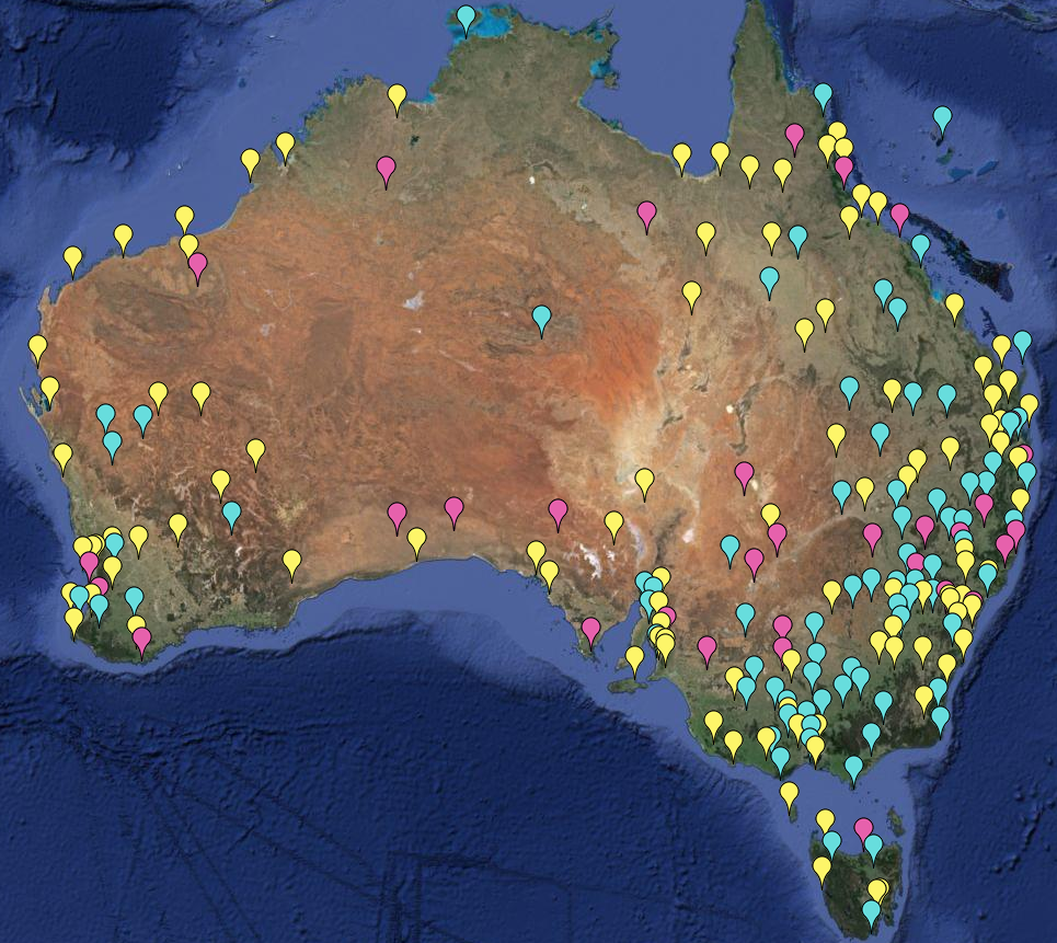
The first link included a gadget using a Google Maps interface that could selectively show stations that were warmed or cooled by adjustment, and by how much. I'll describe it more below the jump, but the original had more complete information. It works for anywhere in the world, but here is an image of Australian GHCN stations with more than 50 years of data. Pink are cooled by GHCN V3 adjustment, cyan warmed, and yellow have no adjustment (strictly, zero trend change):



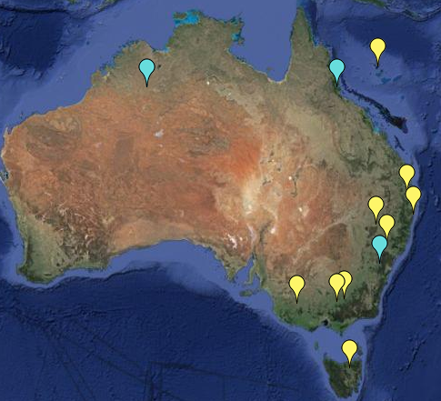
Update: Here is a further plot of the more extreme trend adjustments, magnitude >1 °C/cen. Note that it is for mean temp, not minimum. Amberley still qualifies (1.36°C/cen), but not Rutherglen. Yellow warming; cyan cooling.



The gadget works by "or" logic, which can be tricky. It's better to change than add. To make the pic, I first pressed the Invisible button to start with blank screen. Then I unset the All button, and:

1. entered trend change < 0.0001, pressed the radio button for that, and clicked yellow. All stations with zero or cooling are shown.
2. Then I change 0.0001 to -0.0001 and click pink. Actual cooling trends turn pink.
3. Now I change to > 0.0001 and click cyan. That produces warming trends.
4. Finally I limit to 50+ years. I unset the radio button for trend, set it for duration, and set that to <50. Then I press invisible.

Adjusting Amberley - as it must be

In my last post, I commented briefly on a kerfuffle about adjustments at Amberley. An issue was being made, at WUWT and elsewhere, of the fact that the minimum had been adjusted so that a small cooling trend turned into quite a large warming trend. This made it into the Australian, and the BOM was prressed for an explanation. They pointed out, as I noted there, that there was a large change in 1980, with no associated metadata, which was presumably due to a move within the site.

Now WUWT, following JoNova, is pouring scorn on BoM, saying basically that they are making it up, since they don't have a record. But there is a very good reason why they don't have a record. It wasn't then a BoM site. It was Air Force, and they get the records from them. And the RAAF has its own priorities.

However, the need for the change, and the amount, is obvious if you just look at neighboring stations, and the BoM program did. I'll show this below the jump.

BoM has all the unadjusted data you need, starting on this page. Ask for the kind of data (monthly, mean min etc), with Amberley in the matching towns. Under Nearest Bureau stations, unset the "only show open" button, and it gives the nearest stations with that data. I want stations with data from 1975 to 1985; enough to see what is happening around 1980. The nearest with this data are Ipswich, Samford and Brisbane. I didn't include Mt Glorious because it is on a mountain top; the others are pretty much on the level.

I then subtracted the monthly means for that decade, to remove seasonality. So here is the graph:

It shows the fitted lines, with trends over the decade shown in the legend. Note that the red Amberley curve is pretty much above everything before 1980, and below soon after. The other stations track each other well. Here is tabulated the trends in °C/century. Notice that one of these is not like the others.

Amberley	-15.56
Ipswich	2.23
Samford	5.85
Brisbane RO	2.31

Update. To show the contrast more clearly, and following a suggestion from Victor Venema, here is a plot of the same data, but with the Ipswich values subtracted - ie relative to Ipswich (chosen because it is by far the closest to Amberley):



The fact that Amberley crosses the axis during 1980 is now much clearer.So I added an adjustment of 1.4°C after Jan 1980. Let's see what it looks like now:

Interesting. Amberley is now back tracking the others, except for some disturbance during 1980. And the slope matches the others. But it's irregular during 1980. That means I haven't guessed the date quite right. I've adjusted upward too early. About August 1980 looks right. Here we go:

Yes, that did it. Now tracking the three neighbors very well. And yes, the slope has gone from -15.6 to 3.51, right in the mid-range of the neighbors.

Where did I get 1.4°C? It's a linear calc - to bring the slope back to mid-range. How does this affect the whole trend for Amberley? It increases the trend by 2.86 °C/Cen. Apparently the BoM adjustment was 3.5°C/cen. I'm sure they looked at more stations.

So there you go. The change happened in August 1980, and it dropped temperatures artificially by 2.8 1.4°C.

Amberley, BoM and WUWT

WUWT has a post about Amberley. Amberley is part of the high quality Australian network ACORN. You can scroll down that catalogue to see pictures and description of the site. I've been hearing rumblings about Amberley for months - now apparently Jennifer Marohasy has persuaded Graham Lloyd at the Oz to run a story on how Australia's temp record is being corrupted.

It's of course a familiar story, and Lloyd doesn't need much persuading. It is of course a cherry-pick; even more so since what is shown is the plot of minimum temps; max temps would show only half the effect.

WUWT readers are very short of information here. Lots seem to think that the BoM has obliterated the original data, despite the post featuring a plot of original vs adjusted. So I thought I would try to help, with the following comment:

Mark Addinall says: August 23, 2014 at 9:42 am
"If anyone cares to remember I did that analysis some four years ago. Back when the raw data could still be had over the web. Data has gone."

It hasn't gone. It's all there, as originally reported, at ghcn unadjusted. There is even, normally, a complete accounting, with the effect of GHCN adjustments shown Amberley here. I'm pretty sure you can get unadjusted from BoM too.

Pamela Gray says: August 23, 2014 at 9:58 am
"This is germane to the brief discussion I had with Leif. He asks to be pointed to a temperature record data set used for research purposes that is valid and reliable. My response was that there were none to my knowledge."

Again, GHCN unadjusted has the original data. Go to Daily if you want lots of it. I have an index, TempLS, which works directly from this data.

Anyway, about a week ago I was put on a two-day time-out (circumstances described here). It still persists, and my posts still disappear when I submit them. Twelve hours later, still no show - saga described here.

On the actual adjustments, if you follow the GHCN graphic for Amberley that I tried to link WUWT to, it shows the adjusted and unadjusted (min/max average), and the actual adjustments. There's only one major one, in about 1980. But because the record at 70 yrs is relatively short, it has quite a big effect on the trend. BoM say they don't know what happened, but you can see in the unadjusted a dive around that time, and apparently when compared with neighboring stations, it didn't seem to be climate. Amberley is on the fringe of Brisbane, so there is plenty of data nearby.

I referred in my WUWT offering to a possible BoM source of unadjusted data. I have now located it. It isn't very convenient; you are supposed to input search data for each station and display a graph or table. And they do only min and max; no average.

I've been building up a BoM portal, and I thought this would be a useful addition. I've done it in the first instance for the BoM 2012 HQ network. This is basically ACORN plus some long record stations that have terminated. I downloaded the list from David Stockwell, where there are more details.

So table below the jump, presented in the hope that people will compute more representative cases.

Founding Greenpeace

I've been arguing at WUWT. Quite a few Moyhu posts begin that way, but this time, I've been sin-binned. I must be the first at WUWT to be binned for the offence of querying the accuracy of a Greenpeace publication.

Apparently, I'm still a paid troll. So I guess I should regard it as long service leave :)

Anyway the topic was Patrick Moore. WUWT claims him as a co-founder of Greenpeace. I drew attention to a letter which he wrote in 1971, introducing himself to the “Don’t Make a Wave Committee”, and asking about sailing on the upcoming voyage of the Greenpeace.

Now it seems very odd to me to be writing such a letter to an organisation you are supposed to have founded. Something didn't add up.

So, argument ensued. The principal grievance seems to be that Greenpeace is disowning him because of his change of views, and current activism in contrary causes, as shown by WUWT's enthusiasm for his tour of Australia. More of that later. Greenpeace's currently unfavorable view is expressed here.

Patrick Moore's own view is expressed here. I must say that as an account of the history, it seems to be fair enough (except perhaps to Paul Watson), and obviously he was there. So I quoted almost exclusively from it at WUWT (and here).

July GISS Temp down by 0.10°C

GISS has posted its July estimate for global temperature anomaly. It fell from 0.62°C in June to 0.52°C in July. TempLS declined by a slightly smaller amount. This is definitely more moderate than the high temps of May.

The comparison maps are below the jump.

Here is the GISS map:



And here, with the same scale and color scheme, is the earlier TempLS map:

Previous Months

June
May
April
March
February
January 2014
December
November
October
September
August
July
June
May
April
March
February
January
December 2012
November
October
September
August
July
June
May
April
March
February
January
December 2011
November
October
September
August 2011

More data and plots

TempLS global temp down 0.066°C in July

TempLS dipped in July; from 0.577°C (June) to
0.511°C.

Here is the spherical harmonics plot:



Hot in Europe and E Siberia, cold in Central Siberia and cool in central US. I have o say it looks like a Polar vortex pattern.

Here is the map of the 4185 stations reporting:

CO2 accumulation accounted for by emission and land use

In a previous post, I showed the accumulation of mass of carbon (as CO2) in the atmosphere (using annual Mauna Loa data with Law Dome ice core data), on the same scale as the mass of carbon as fossil fuels (and cement making) that we have emitted. It makes it very obvious that the rise in CO2 is associated with our emission, and that we have at most stages emitted more than has accumulated.

However, the match is not exact. The CO2 did start to rise while our emissions were small. I remarked that this is likely due to land clearance, which transfers C from the plant biomass to air. A commenter suggested that I include that in the plot.

So I do that here. I am using the land use data of Houghton, from the CDIAC site. It goes from 1850 to 2005. I have assumed for plotting that annual increments since 2005 are unchanged (they were fairly stable pre-2005). It is an estimate of nett carbon emitted due to land use changes in general, including reforestation etc.

This allows me to do a separate calculation of the airborne fraction (AF) - the fraction of emission that stays in the air. I find that the added CO2 rises very linearly with total anthropogenic addition, and the AF is 44%, with very little sign of change.

So here is the revised plot of mass of atmospheric C and the anthropogenic additions (see previous post for scale factors). As before, the light red curve shadowing observed C is the anthro added C, scaled by AF of 0.44.


There is a slight dip in ice core CO2 1600-1800, which could be due to the LIA,


Below the jump I'll show a plot for more recent years, and the airborne fraction plots.

Here is the recent version, post 1800:



And here you see, for the Mauna Loa period (1959-), the mass of C in the air plotted against all anthro addition (fossil + land use). It is very linear, and the regression slope is 0.439.



Airborne fraction is described in AR4 Ch 7. It is often described in terms of AF of emissions, rather than total anthro. Here is my corresponding plot of air C vs fossil fuel emissions.



The AF is of course larger, at 55%, and is quite close to what Scripps quotes.

A point is that my values seem much stabler with lower errors than the AR4 values. I think the method they describe, showing the ratio of annual changes in isolation. loses a lot of information - the fact that the changes are consecutive and cumulative. In effect, they treat AF as something that could be different with no correlation from year to year, and they describe population statistics of the implied values. My analysis assumes that the AF is a physical thing, likely to be sustained from year to year.