This post is a follow-up to one
a few days ago on differences seen calculating monthly global averages using
TempLS and
version 4 of GHCNrather than V3. It followed a
post of Clive Best, who has a similar program, and was finding differences. I too found that June 2019 rose about 0.07°C while using GHCN V3 did not show a rise. I think overall differences are small, but I wanted to look at the underlying arithmetic.
So, as
foreshadowed, I adapted my program to use its
LOESS based calculation and
graphics, in which I could calculate differences. But there was mission creep, as I found that being able to put disparate data on the same equally spaced grid made a lot of other things possible. So I showed also the effects of homogenisation. It does answer the question of why V4 made a difference this month, but there is a lot more to learn.
First let me tell the many uses of the main graphic, which is shown below. It is the familiar
WebGL trackball Earth. You can drag it about and zoom. Click on the little map to quickly center at a chosen point. But importantly for this inquiry, you can control the content. The checkboxes top right let you switch on/off the display of V3 and V4 or SST nodes, or the shading (called "loess"), or even the map. And the radio buttons on the right give the choice of five data sets for June 2019, which are
- Un V4-V3 which is the difference of TempLS anomalies using unadjusted GHCN data from V4 and V3.
- Adj V4-V3 the corresponding difference using adjusted GHCN data (QCF, pairwise homogenised)
- V4 Un - Adj the difference between unadjusted and adjusted data, for a V4 calculation
- V3 Un - Adj same for V3
- V4 Unadjusted just the TempLS anomalies using V4. It is the LOESS version of my regularly updated mesh plot.
So I'll show the plot here, with below an expanded discussion of what can be learnt from it.
Improved coverage in GHCN V4
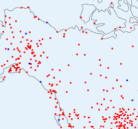
This is shown most clearly if you switch off loess, and toggle the boxes controlling V3nodes and V4nodes. What are displayed are the stations that reported in June (so far). The improvement of coverage is greater than I had thought, and as I will show is the basis for V3/V4 discrepancies.
The V3/V4 difference for June, and reasons.
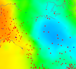
One thing that surprised me was the coherence of the difference plots. The LOESS does some smoothing - you can estimate the effect by looking at the smudging around coastlines. The SST is the same between versions, so color in the sea means either islands or smoothed land. It fades basically exponentially, so color difference tends to exaggerate the spread. It's surprising because you would expect that station differences between V3 and v3 would be fairly random.
But only if both types are represented, and that is the key here. There is, for example, in Un V4-V3 a big warm patch around Senegal. I'll show also the station distribution and the anomalies:
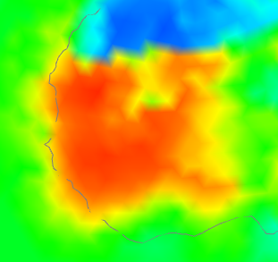 | 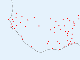 | 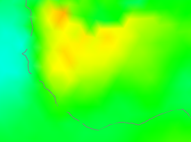 |
| V4-V3 difference | V4 stations | V4 anomaly |
I haven't shown the V3 stations, because basically there aren't any (check the figure). So how did V3 cope? It used information from nearby, a lot of which was sea. V4 had much better coverage, so the region is predominantly represented by land. And as the third column choes, the land was warmer, by anomaly. Not a lot, but watch for the different color scales here. The apparent warmth in the first column is a much smaller temperature difference - the scales are about 4:1.
So here is where a discrepancy arises - an area which V4 covers much better, which happened to be warm that month. Here is an example going the other way in NW Canada:
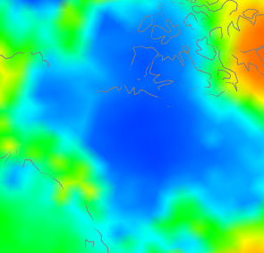 |  |  |
| V4-V3 difference | V3 and V4 stations | V4 anomaly |
have shown the same tableau, but this time the centre plot shows V3 stations as well (in blue) since there are a few. But not many. Again what is happening is that the rather faint blue patch on the right, because it is picked up by V4 but hardly by V3, turns into a V4-V3 discrepancy on the left. One more case - Antarctica:
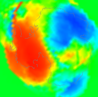 |  | 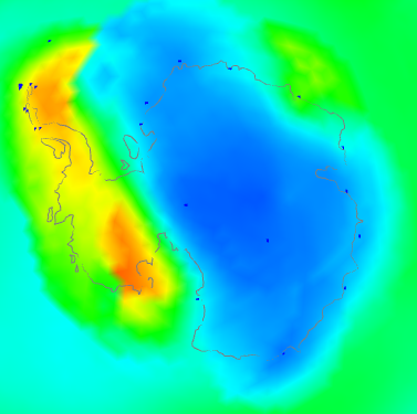 |
| V4-V3 difference | V3 and V4 stations | V4 anomaly |
This is a bit of both. It shows a discrepancy plot warm (ie high V4-V3) in the W, opposite in the East. The station plot shows a big increase in coverage in the interior, and also on the peninsula. And the right shows that the actual anomaly was also strongly divided between W and E. You might ask - why did the strong warmth in the East show a relatively small discrepancy? I think it is because although the V3 stations were sparser, they did give reasonable coverage around the coast of EA. So although the interior had to look far afield to infer temperatures, mostly it found land rather than sea.
So overall I think that is the cause. There are a few regions around the Earth where V4 has much better coverage. If these happen to align with anomaly patterns, those patterns will be reflected in the V4-V3 difference, and because there are only a few, from time to time they will align by chance.
I think this also explains the small persistent long term changes. As warming proceeds overall, it will more often happen that the anomaly patterns in V3-sparse areas with vary from SST on the warm side, producing a warm V4-V3 difference, which will accumulate.
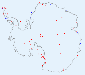
What about adjusted data, which seems to show a little more warming? I think it just fixes some aberrant cases which would reduce the effect in unadjusted data. Here is another tableau from Antarctica
| 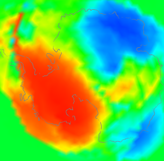 | |
| Unadjusted V4-V3 | Adjusted V4-V3 | |
The unadjusted had a number of blue spots along the Antarctic peninsula. Homogenisation identified some of these as biases that could be corrected. Whether right or wrong, the arithmetic result is of a discrepancy that integrates to a higher value, because of reduced noise.
To summarise, I think the reason is not that V3 stations were reporting temperatures different to V4; it is that in some regions they weren't reporting temperatures at all, and the discrepancies are a resulting artefact. So where it happens (not much), V4 is better than V3. This may not affect methods like HADCRUT and NOAA in the same way, since they more rigidly separate land and sea. But I think Clive's method will respond in the same way as mine.
Coverage patterns
Again, to see this I'd recommend switching off loess, and then between V4nodes on and V3nodes on. I was actually surprised at how many areas in June were much better covered by V4. Large areas of Africa like the Senegal area above, are much better. There are, of course, still gaps. Antarctica is much better in the interior. Australia is better, and so is the Amazon region.
Adjustment patterns
I'm looking now at radio buttons 3 (V4 Adj - Un) and 4. If you look at the color keys, the adjustments are quite small. I was a bit surprised that there are any at all. So it probably isn't that useful to talk much about June, since it is in older times that adjustment has more effect. Still, June is what we have here - I may try and look at more data in a later post.
Again the patterns are mostly quite striking. The US is an exception,
where there may be a residual effect of TOBS adjustment (no TOBS is done - thanks, Steven). Africa is an interesting case, where two large regions are warmed, and one is cooled. The Amazon is cooled, but further south is warmed. China and Thailand are warmed.
Button 4 (V3 Adj - Un) shows the corresponding pattern with V3. This time North America is mostly warmed. The Arctic ocean (from land stations) is cooled. Africa is more cooled than warmed. N China and west are warmed, but not the south. W Antarctica is cooled.
I don't want to go too much further into this, as I don't think the most recent month is the best place to look for adjustment effect. I'll hope to do more.
More plot details.
Usually I show the actual mesh being used for shading. That isn't so important here, but if you want to see it, and read more about the icosahedral mesh which underlies the Loess method, it is described
here.
Being V3 (I will write up) of the WebGL facility, there is improved zooming, with buttons as well as right button motion.
The Match button enforces the same color scaling, but I don't think that is wise here. I haven't included station names, so clicking won't bring them up. The data file is already over 1 Mb, and it would be messy with the two station sets.


technically V4 does not do a discrete TOBS adjustment. TOBS only gets done for USHCN.
ReplyDeletein v4, since its global and since there is not good global metadata on TOBS, Pairwise Homogenization
is the only method used.
Thanks, Steven
DeleteI wrongly thought they took in TOBS-adjusted data. I'll correct
Excellent post, Nick. The graphics are impressive, although with LOESS switched off nothing at all appears on the map that I see: the station locations are missing, however I toggle the V3nodes, V4nodes and SST buttons. I've tried in both Firefox and Chrome.
ReplyDeleteI'm surprised that v4 shows much higher warming in West Antarctica than v3. There are only a very limited number of stations there and their records have been readily available for many years. Moreover, there is essentially no continuous record available in the interior of W Antartica that stretches back to before 1980. Do you know if GHCN v4 has followed GISS and BEST in using the unhomogenised Bromwich et al composite reconstruction at Byrd, which basically stiches together the manned Byrd station record that covers 1957 to the early 1970s with the 1980 on automatic Byrd station record, with no offset despite their differing location, construction and local environment? That reconstruction shows a high warming trend, but its method is inconsistent with normal homogenisation approaches (and is in direct conflict with BEST's 'scalpel' method).
Thanks, Nic.
DeleteSorry about the troubles with the checkboxes. I could try to diagnose that - if after a failure in Firefox you click on Ctrl Shift K, you should see a debug window, and the console tab will bring up a list of error messages. Ctrl shift I is similar in Chrome, and may make the error clearer. There will be junk from the various hitches with the Google system, but probably the top message will be the key one. It should give the line number where the fault is.
I don't know the details about Byrd etc, but V4 does have more stations. I have another graphic here in similar style which shows the V4 stations, this time with a triangle mesh. On this version you can click on station locations for more details.
Thanks, Nick
DeleteI clicked on Ctrl shift K in Firefox and theis non-Google error shows first:
‘src’ attribute of [script] element is empty. why-is-this-june-hotter-seen-with-ghcn.html:612:1
In Chrome, the first error message in the Console on invoking Ctrl shift I is:
why-is-this-june-hotter-seen-with-ghcn.html:875 [Violation] Parser was blocked due to document.write([script])
Hope this helps. Note that I'm now finding displaying the main graphic at all, in both Firefox and Chrome. It works sometimes but not others (possibly a SSL or TLS error - I'm finding that pages using encryption quite often don't load first time?), and not at all for the linked page. The error messages I get in Firefox for that web page are:
Synchronous XMLHttpRequest on the main thread is deprecated because of its detrimental effects to the end user's experience. For more help http://xhr.spec.whatwg.org/ ghcn0.js line 3 > eval:1:3349
Cross-Origin Request Blocked: The Same Origin Policy disallows reading the remote resource at https://s3-us-west-1.amazonaws.com/www.moyhu.org/data/ghcn/new/anom2019_6.js. (Reason: CORS request did not succeed).
‘src’ attribute of [script] element is empty.
Nic
Thanks, Nic
DeleteThat gives me a lot to work with, I'll see what I can do.
Nic,
DeleteAs far as I know, only GISS v3 uses the reconstructed Byrd series. GISS V3 gets the Antarctic data through SCAR.
The reconstructed Byrd is not included in GHCNv3, GHCNv4, GISSv4, or BEST.
Here is BEST's own Byrd "reconstruction" with gaps:
http://berkeleyearth.lbl.gov/stations/166906
South of 60?
ReplyDeleteV4 has 95 stations.
Byrd is two different stations in V4
As you note there is no continuoius record. Dont need them.
Not sure when we make the change over to V4, need to ask Robert.
Interesting Nick,
ReplyDeleteYou are right of course that where there are sparse stations near the coast then the triangulation will pick up one land station and two SST points as vertices. These differences mean that spatial detail will be better in V4 than V3. However, I am more concerned about systematic adjustments made to the underlying station data.
To check this I restricted the calculation of the monthly and annual temperature of V4 to only their versions of V3 stations. If the station data were the same then I should get back the V3 result. I don't - I get the V4 result. The underlying Tav values in V4 are different to those in V3. That is the problem!
http://clivebest.com/blog/?p=8981
Clive,
DeleteIt didn't seem to me that you did quite get the V3 result. It's close recently, but not so much further back. And I wonder about whether the subsets match. If more stations from the V4 subset of the 3500 report than of the V3 subset, there is still a version of the discrepancy here.
I'm planning a test that you could probably do too. Suppose you have done a V4 mesh analysis; you have nodes Z4, anomalies A4, with mesh M4 and weights W4. And from V3 also Z3, A3 etc. Then with M4, interpolate A4 onto Z3, with result X. Then X.W3 should match the V3 average A3.W3, rather than the V4 average A4.W4. Maybe you don't explicitly use weights; then it would be the corresponding integration procedure.
"I get the V4 result. The underlying Tav values in V4 are different to those in V3. That is the problem!
DeleteErr that is how pHa works.
V4 has more stations than V3. When you do pairwise homogenization you have to collect
all the highly correlated neighbors. A station in v4 will have more neighbors than that
same station in v3.
Next, the SNHT process will identify those stations and their points in time when
they disagree with thie neighbors. Increase the neighbors and these points will change.
This comment has been removed by the author.
ReplyDeleteClive,
DeleteAre you looking at it with the nodes switched off? The initial picture is red because of node density.
Yes - I realised immediately and blogger amazingly gave me a delete option !
DeleteYou can put it back ;-)