Saturday, July 30, 2011

Missing Lat/Lons in CRUTEM3

I found the latitude/longitude info in CRUTEM3 to be generally better than in some earlier versions of GHCN. There seemed to be fewer cases of stations turning up in the sea - the KML files that I did make this rather obvious.

However, there were some down as missing data. TempLS needs some lat/lon info - perfect accuracy isn't necessary, but for the weighting it needs to know within a degree or so. So I tracked some of them down. None of the stations are major data sources, so they could have been omitted. Many were in a group of Argentine stations from the early Smithsonian data set. But I tracked the lat/lon to an accuracy that was adequate for my needs - below the jump.


The table of missing lat/lon data is here:
85997377254-999SERRO DO PILARPORTUGAL19011930101901
390000535-426-999ZAMETCHINOUSSR19011954101901
685807-296-304-999PIETERMARITZBERGS.AFRICA18701886101870
688607-333-265-999GRAHAMSTOWNS.AFRICA18551870101855
967811-62-10661400TJIBODASINDONESIA19051948101905
968531-79-11291735TOSARITHAILAND19121933101912
969887-79-1149930KAJOEMASINDONESIA19121918101912
999096-341-1180-999BREAKSEAAUSTRALIA18971899101897
999099-999-1999-999LONDONAUSTRALIA18971899101897
999201-346583-999ANGEL GALLARDOARGENTINA19321960101932
999207-391676-999CORONEL J.J. GOMEZARGENTINA19311960101931
999211-346595-999FORTIN MERCEDESARGENTINA19311958101931
999213-391-1672-999GEN. GODOYARGENTINA19321959101932
999216-226623-999 LAS DELICIASARGENTINA19311960101931
999229-246585-999TACAAGLEARGENTINA19311960101931
999236-390681-999VILLA NEUGUESARGENTINA19311960101931

In the table, I've replaced the missing lat/lon (2nd and 3rd cols) by what I think is the coords of the town referred to. Remember that CRUTEM uses negative longitudes. Sometimes there is some ambiguity - for TOSARI, for example, I punted for the mountain town in Java (as suggested by altitude and WMO number).

I couldn't locate LONDON, Australia (it's hard to search for), but there were only two years of readings, so I dropped it. VILLA NEUGUES I assumed was a typo for something involving Neuquen. Tjibodas I tt\ook to be the botanic gargens near Jakarta, and Angel Gallardo the district in BA.

I corrected an error with Clare Post Office. It was entered twice - once with the major set of data, and once with a patchy set, mostly missing , and with latitude of wrong sign. I corrected the latitude, but probably the whole set should be omitted.

There is a lot of altitude data missing (-999), but I don't need it.


Thursday, July 28, 2011

More on CRUTEM3 stations in Google Earth

An update on the previous post.I've realised that I can provide a lot more information by using folders in KML. I have made a file where every station is assigned to a folder according to the year in which data ceased, or 2011 if it is still current. The years are then grouped into folders of a decade or so.

The use of this is that in Google Earth, you can make the folders and subfolders invisible (hierarchically). On the left, near the top, there is a box called places. If you have brought up the station KML file, there will be a box called Temporary Places. If you open that you'll see the filename (crutem_end.sav), and below that you can expand to show the directory. Beside each entry is a little screen that you can click to toggle visibility.

So if you want to see which stations disappeared in the '80's, just blot out all other top folders. If you want to see what happened in 1988, go down to that level. If you want to see all current stations, blot out everything except 2011. And so on.

There is another file (crutem_start.kml) foldered according to start year, which you can treat similarly. It is an interesting historical exercise to click through as the US, say, gets populated with stations in the 1850's.

I'll put up similar GHCN files to replace the less efficient ones from last year. I've replaced the contents of the crutem_all.zip file with these.

CRUTEM3 stations in Google Earth

I've made KML files for the CRUTEM3 stations. They are on the document store as crutem_kml.zip. If you just extract the files, you'll find two kml files - crutem_all.kml and crutem_recent.kml. The first shows all stations that have reported since 1900, and the second stations that have reported since 2000.

They show up as yellow pushpins - the size indicates the total years in the record. CRUTEM3 stations have longer durations than GHCN - so the largest size is over 90 years, and the smallest under 50. There are, in the inventory, 1943 stations over 90 years, 1198 under 50, out of a total of 5112. This is the count of lines in the record - it overstates the length because there are some years entered in the file with no data. (Update - it seems I was wrong about that - it's not overstated).

If you click on a station a flag pops up with a few more details. Here is a sample view of stations that have reported since 2000:


A first look at CRUTEM3 station data

CRUTEM station data has been released as noted  here. I'll be doing a run of TempLS to check what sort of global averages and trends it produces, with comparisons. And I'll try to produce some Google Earth files.But firstly, just some station numbers data and maps, below the jump.

The general layout of the file is easy to use. They mix the inventory data with the temperatures, which takes some sorting out. For some reason, they give negative longitudes.


On station numbers, here is a plot of how they have varied since 1900. There is not much very recent data - it fades about 2007-8. This plot shows stations that reported at least once in each year.


Heere is a graph showing recent data better. It is of course heavily influenced here by the GHCN history.


Now I'll show station maps from various perspectives. First a set of stations that have reported some time since 1900:


Now looking at stations that have reported since 2000:


Finally, a look at station that have reported since 1980:


Saturday, July 23, 2011

Using RghcnV3 - a very simple TempLS

I've been experimenting with Steven Mosher's R package RghcnV3. It has many useful features, and I think the R package format serves it well. I'm not as enthusiastic as Steven about the zoo and raster structures, at least for this purpose, but still, I may yet be convinced.

Anyway, it certainly gets some of the messy initial data structuring out of the way. So since I am currently working on Ver 2.2, I thought I would put together a very simple version using some of the more recent ideas, in the RghcnV3 style.
Update - I've added a version of the code with detailed comments at the end.


TempLS basics

Firstly, a reminder of how TempLS works. After data rearrangement, we have an array of temperature readings, over some number S of stations, and over M months (usually 12, but can do seasons etc) and Y years. This is a SxMxY array with many missing values.

I'll explain the math in a similar style to this account of V2. I'll use a notation, described there, in which arrays (matrices etc) are represented with suffixes, and equations including them are true for the natural range of values. To save summation signs, I use a summation convention in which a repeated index is assumed to be summed over the range. But to emphasise that, I use colors. Summed indices are blue, independent ones are red. There are some I need to exempt from the summation rule, and these are green.

So we assume that the observed temps x can be modelled with
  • a local temperature L, which varies over station and months, but not over years. Think of it as a monthly average, and
  • a global temperature G uniform over months and stations, but varying with years. This corresponds to the global anomaly that we are after.
So we write a model equation

xsmy  ~  Lsm  +  Gy
I'll repeat here the least squares part from that earlier post. It's useful to maintain a convention that every term has to include every red index. So I'll introduce an identity Iy, for which every component is 1, and rewrite the model as
xsmy  ~  IyLsm  +  IsmGy

Weighted least squares.

The L and G are parameters to be fitted. We minimise a weighted least squares expression for the residuals. The weight function w has two important roles.
  • It is zero for missing values
  • It needs to ensure that stations make "fair" contributions to the sum, so that regions with many stations aren't over-represented. This means that the sum with weights should be like a numericam integral over the surface. w should be inversely proportional to density.
So we want to minimise w(smy)(xsmy - IyLsm - IsmGy)2

Differentiation

This is done by differentiating this expression wrt each parameter component. In the summation convention, when you differentiate a paired index, it disappears. The remaining index goes from blue to red. The original scalar SS becomes a system of equations, as the red indices indicate:
Minimise:w(smy)(xsmy - IyLsm - IsmGy)2
Differentiate wrt L:   w(smy)Iy(xsmy - IyLsm - IsmGy)
Differentiate wrt G:w(smy)Ism(xsmy - IyLsm - IsmGy)
Notice what we have here - linear equations in L and G, and all we need is the data x and the weights w.

Equations to be solved

These are the equations to be solved for L and G. It can be seen as a block system:
A*L + B*G  = X1
BT*L + C*G  = X2
combining s and m as one index, and where T signifies transpose. Examining the various terms, one sees that A and C are diagonal matrices, so the overall system is symmetric.

The first equation can be used to eliminate L, so
(C -  BTA-1B)*G = X2  -  BTA-1X1
This is not a large system - G has of order 100 components (years).

Implementation with RghcnV3

There are just three steps. We have to get the array x. RghcnV3 can get us (as explained in the manual as far as the output of readV3Data(). This is a large array ordered first by months (in rows), then by year, then by station. There is then a function v3ToZoo() in V1.3) which should get it into a structured array. Unfortunately, I ran out of memory at that stage. But the further rearrangement was a basic step in TempLS, so I used the sortdata() routine to do that. The arguments are the data array, and a vector with the start and end year of the period you want to look at.The resulting x array is ordered as suggested above, by station, month and year.

Weighting

Then we need a weight function w. A basic method is to divide the surface into 5x5 lat/lon cells, and get a station density by dividing the area of each cell by the number its stations reporting in each month. This is done in the routine makeweights, which returns the array w.

Solving

So that's it. We have the needed w and x; the rest is just some summing over rows etc to get the block matrices, and then a block inversion. This is done in the routine solveTemperature, which returns the temperature anomalies about a mean zero. I've added a plot statement.

The code

As promised, just three routines. Start with dat, the array from readV3Data(), and your choice of years yrs[1:2]. There is another version with detailed comments below:

sortdata = function(v,yrs=c(1900,2010)) # Sorts data from v2.mean etc into matrix array x
{
nd=dim(v)[1];
y0=yrs[1]-1;
iq=c(0,which(diff(v[,1])>0),nd);
jq=length(iq)-1;
x=array(NA,c(jq,12,yrs[2]-y0));
for(i in 1:jq){ # loop over stations
kq=c(iq[i]+1,iq[i+1]);
iy=as.matrix(v[kq[1]:kq[2],]);
oy=(iy[,2] > y0) & (iy[,2]<=yrs[2]);
if(sum(oy)<2)next;
iz= iy[oy,];
x[i,,iz[,2]-y0] = t(iz[,3:14]);
}
x;
}

Then the routine to make the weights - needs x and lat/lon:
makeweights = function( x, inv)
{
d = dim(x); wt = array(NA,d);
ns = floor(inv$Lat/5)*72 + floor(inv$Lon/5) + 1333;
wtt = sin((1:36-0.5)*pi/36);
w_area = rep(wtt,each=72);
for(i in 1:d[2]){
for(j in 1:d[3]){
ow = !is.na(x[,i,j]);
n=ns[ow];
kc=tabulate(c(n,72*36));
ok=kc>0; wc=w_area;
wc[ok]=w_area[ok]/kc[ok];
wt[ow,i,j]= wc[n];
}
}
wt;
}

Finally, the solve routine:

solvetemperature=function(wt,x)
{
wt[is.na(wt)]=0;x[is.na(x)]=0;
x=x*wt; d=dim(x); d=c(d[1]*d[2],d[3]);
dim(x)=dim(wt)=d;
A=rowSums(wt)+1.0e-9;
R1=rowSums(x);
C=colSums(wt);
R2=colSums(x);
aw=array(rep(1/A,d[2])*wt,d);
b = drop(R2-R1 %*% aw);
S=diag(C) - t(wt) %*% aw;
S[1,1]=S[1,1]+1; # there is a dof to be fixed
y=solve(S,b);
y-mean(y);
}

And the program to run it all:

x=sortdata(dat,yrs);
wt=makeweights(x,inv);
T=solvetemperature(wt,x);
png("TempLSv0.png",width=500);
plot(yrs[1]:yrs[2],T,type="l");
dev.off()

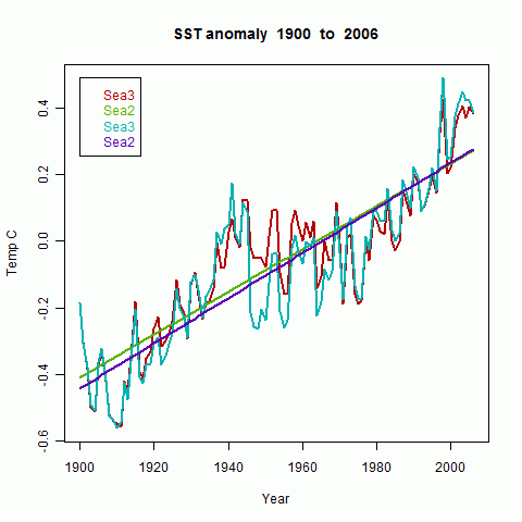
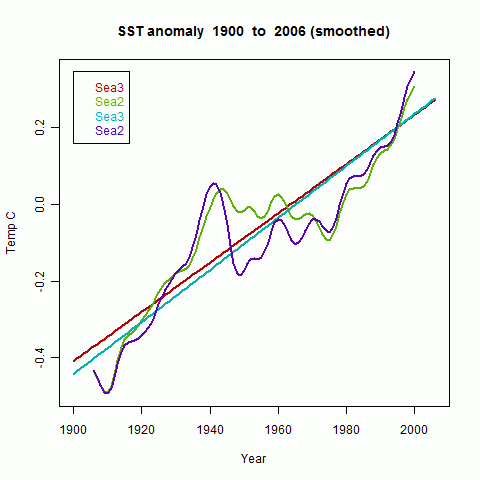
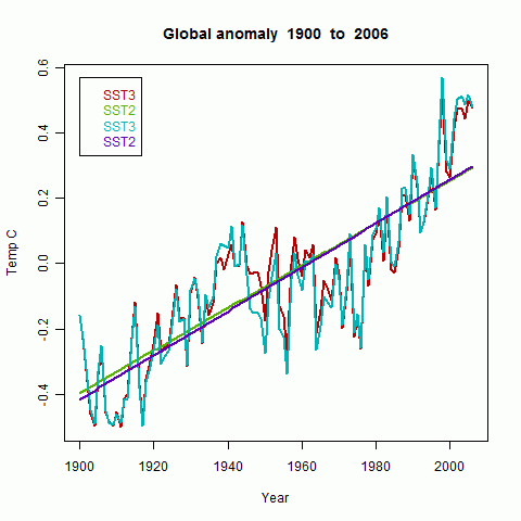
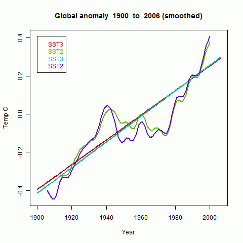
And a (no-frills) result:


Here is a version of the code above with line by line comments.

#You'll want your own version of yrs
sortdata = function(v,yrs=c(1900,2010)) # Sorts data from v2.mean etc into matrix array x.
#v is just the v3.mean file read in - one year per row, one station block after another. Within a block, the years are in order.
{

   nd=dim(v)[1]; # Number of stations in inventory
   y0=yrs[1]-1; # Year zero
   iq=c(0,which(diff(v[,1])>0),nd); # Endpoints of each station block of data (where the stat num ber increments)
   jq=length(iq)-1; # Number of stations in data set
   x=array(NA,c(jq,12,yrs[2]-y0)); # setting up the big temp matrix
   for(i in 1:jq){ # loop over stations
       kq=c(iq[i]+1,iq[i+1]); # marks the block of station i
       iy=as.matrix(v[kq[1]:kq[2],]); # copies that block of info
       oy=(iy[,2] > y0) & (iy[,2]<=yrs[2]); # selects the years within range
       if(sum(oy)<2)next; # reject stations with less than a year of data (can't get an anomaly with 1 dof)
       iz= iy[oy,]; # the selected block
       x[i,,iz[,2]-y0] = t(iz[,3:14]); # copy into x
   }
x; # return x
}#;
makeweights = function( x, inv)
# To return wt, a matrix with the same structure as x
#ie a weight for every station/month/year, but zero or NA if missing
{
  d = dim(x); wt = array(NA,d); # set up the big blank
  ns = floor(inv$Lat/5)*72 + floor(inv$Lon/5) + 1333;
# ns lists a (5x5 degree) cell number for every station in the inventory
  wtt = sin((1:36-0.5)*pi/36); w_area = rep(wtt,each=72);
# w_area is an area weight for each cell
  for(i in 1:d[2]){ # loop over months
    for(j in 1:d[3]){ # loop over years
       ow = !is.na(x[,i,j]); # which stations reported in i/j
       n=ns[ow]; # and what were their cell numbers
       kc=tabulate(c(n,72*36)); # frequency of cell numbers
       ok=kc>0; # logical for empty cells (that month)
       wc=w_area; #Initialize the weights to the areas
       wc[ok]=w_area[ok]/kc[ok]; # now divide the weights by number of stats, to get inverse density
       wt[ow,i,j]= wc[n]; # set the weights for that i,j
    }
   }
 wt; # return the big weight matrix
}
#Now we have the weights wt and temp matrix x, can solve linear systen for temp anomaly
solvetemperature=function(wt,x)
{
# to avoid NA fuss, missing readings have zero weight, so temp doesn't matter
   wt[is.na(wt)]=0;x[is.na(x)]=0;
   # redimension to a matrix with s&m vs year
   x=x*wt; d=dim(x); d=c(d[1]*d[2],d[3]);
   dim(x)=dim(wt)=d;
   A=rowSums(wt)+1.0e-9; # Top left diag block matrix
# There can be missing lines with all zero. Instead of eliminating them, just add something to the diag to avoid a 0/0 error. No effect on result.
   R1=rowSums(x); # Corresponding RHS
   C=colSums(wt); #Bottom right diag matrix
   R2=colSums(x); # Corresponding RHS
   aw=array(rep(1/A,d[2])*wt,d); # LHS term after dividing by A to eliminate L
   b = drop(R2-R1 %*% aw); # Elimination op for RHS
   S=diag(C) - t(wt) %*% aw; # Local temp has now been eliminated, along with variables s and m.
#Now the equation is just in yearly T anomalies over years. Symmetric.
# S is singular, because an arbitrary constant could be added to G and subtracted from L.
# So arbitrarily set anomaly 1 to zero
   S[1,1]=S[1,1]+1;
# Now solve - S could be up to 150x150 say (yr[2]-yr[1])
   y=solve(S,b);
# Now reset to mean zero (fixing that arbitrariness)
   y-mean(y); # zero mean anomaly returned.
}
# End functions.
# Execution You start with v from data file (readV3Data()) and inv from inventory (readInventory())
# All you need from inventory is lat/lon
x=sortdata(dat,yrs);
# Many other makeweights() are possible
wt=makeweights(x,inv);
T=solvetemperature(wt,x);
# A simple plot on a png file; comment out to see on screen (also dev.off())
png("TempLSv0.r");
plot(yrs[1]:yrs[2],T,type="l",xlab="Year");
dev.off();


Friday, July 22, 2011

TempLS V2.2 and the June 2011 global average

I'll soon be releasing Ver 2.2 of TempLS. Its main new features are:
  • An ability to model global temperatures with monthly resolution, rather than annual. You can also ask for a selection of months - say, summer.
  • The graphics is internally reformatted so that each plot is generated by a function from a data list, which is available after the run. That means that plots can be tweaked, merged etc.
  • Instead of providing just one data set and inventory, you can provide several, and they will be merged. In practice, at the moment, that means that land sets (eg GHCN2, GHCN3, GSOD) and SST sets (HADSST2, HADSST3, ERSST) can be combined as desired. That will allow comparisons (a future post). It's also easier to mix in, say, USHCN.
  • A new weighting function. Previously there was uniform, 5x5 lat/lon cells, and the adaptive methods ( triangular mesh and Voronoi). The complicated ones are good, with one cell for each station in each month, but time-consuming. So I made a new one, which has latitude bands of near-squares, but added the capability that empty cells would have potential weightings distrubuted among neighboring cells that do have stations (those stations are upweighted). This removes the bias caused by empty cells.

A lot to write about, but for the moment, I'm exploiting the ability of the monthly scheme to report the current month. Fixing bugs kept me from getting ahead of the majors this month, but maybe next. I've added TempLS to the regularly monitored set.

The spatial methods work, too, and I'll show a comparison of June with Gistemp below the jump. But here's the most recent time series plot:


These anomalies are set (for plotting) to a common base period of 1979-2000. Raw numbers from TempLS are on a 1961-90 base. And here is the monthly plot for the last four years.

These plots were done using GHCN v2 and HADSST2. Soon I'll do a post with GHCN v3 and HADSST2/ERSST.

The spatial analysis was done using as series of about 12x12 spherical harmonics. It isn't as detailed as the Gistemp one that follows, but gets the main features right.


And here is the GISS comparison.


In a future plot, I'll set out the least squares theory for the monthly adaption.

Sunday, July 17, 2011

NOAA for June - up from .497 to .579

The NOAA June global surface temperature anomaly is out now - up from 0.497°C to 0.579°C. That's quite high.

I don't normally post for each monthly temp, but I wanred to mention this one, because it's the first new monthly reading since I put up the monitoring post. And yes, it shows up in bold as I hoped it would. I'll try for colors next.

I was also watching carefully because I'm about to post a new version of TempLS (V2.2) which among other things will allow TempLS to produce real-time readings, probably quicker than NOAA. But for that I have to use ERSST data, which is prompter that HADSST2. I'm less familiar with it, and I'm finding a big dip around 2006. There was a changeover then in using satellite data. Anyway more recent output seems OK. So I'll check a bit more, but if I haven't made a mistake (that I can find) I'll probably post tomorrow.

Thursday, July 14, 2011

Global surface temperature reconstructions with the new HADSST3

Global reconstructions with the new HADSST3

There is a new version of sea surface temperature records: HADSST3. It is reported here, commended here, and criticised here.

The most noted change relative to HADSST2 is in a post-WW2 period when there was an issue with bucket and engine intake readings. HADSST2 was said to have a spurious dip in this period, which HADSST3 corrects. Consequently, trends of SST calculated over the last fifty years, say, have been slightly reduced.

I have not yet seen it used in any global land/sea index calculations. I have seen the effect inferred, but not measured.

Well, this is something TempLS V2.1 can do. So I downloaded HADSST3 from the Met Office site. Currently, it only goes as far as 2006. I compared it with using HADSST2, both in association with land measurements from GHCN v2.

Since the effect on trend has been a point of argument, I've made a plot of the trend calculated between 2006 (last year of HADSST3 currently) and years starting before about 1990, going back.
Update - I've added a table of trend values at the end of the post.
Update - since a lot of blog discussion talks of the % change in trend in using new HADSST3, I've replotted the last two plots of this post (qv) in % terms - change in the trend measured back from 2006, for both the SST average and for global land/sea. Here it is:


The output here is derived from the TempLS standard plots. The HADSST3 source was the HADSST3_median file. Firstly I show the "station" count. That is, the number of 5x5 cells in any year that have at least one monthly measurement. HADSST3 has more, but there is very little difference. The effects of the two world wars are obvious. In the legends "Sea3" or "SST3" refer to HADSST3, etc.


Next the area-weighted means of SST anomalies only, calculated with HADSST3 and HADSST2. As expected, HADSST3 substantially increases the average in the post-WW2 period. There's also a slightly puzzling discrepancy post-2000. ClimateAudit has a plot which is mostly similar, but doesn't have that discrepancy. (Update - I see that RealClimate shows a corresponding plot which does have this discrepancy). The least squares regression line is shown, and also a smoothed version:


Now comes the Global land/sea average, calculated using GHCN v2 means for land stations. The difference is similar, which is expected, since the SST measurements are a dominant component of the average.

>

Here is an expanded version of each (unsmoothed) in the period 1950-2006:


Finally, here is the trend of the global average, calculated back from 2006 to the year shown on the x-axis. As might be expected, there is a minor difference, greatest in the post WW2 years, but less before and after.
Update - for completeness, I've added the analogous plot for SST averages.


Update - here are the numerical trend values corresponding to the plots:
LamdSST2/3 are the global measures, Sea2/3 are the SST's. Standard errors do not allow for autocorrelation.
Trend LandSST3 LandSST2 Sea3 Sea2
1900-2006 0.0649 0.06726 0.06425 0.0678
Trend_se 0.004124 0.00441 0.00359 0.003899
1950-2006 0.09755 0.1169 0.07075 0.09944
Trend_se 0.01056 0.01012 0.009047 0.008181

Wednesday, July 13, 2011

Updating Arctic ice and global temperature data

Since my recent experiments with JavaScript, I've been teaching myself various tricks at w3c Schools. This has sorted out all kinds of modern mysteries for me. They cover JavaScript, HTML and variants, XML, PHP, SQL, CSS and all manner of things I hadn't heard of. And what I really like is that each command has a try-it page where you can tinker with the text and see the results in another part of the window immediately.

Anyway, that encouraged to do something that I tried last year - putting up the latest sea ice and global temperature numbers. But then I did it manually and it got to be a drag. Now I'm hoping I can fully automate it, using R as well. So here's a start. (Though Neven has the full ice story).

The automation mainly consists of an embedded html window in which the numbers will appear. I'm planning to run the script at least once a day, and about 1.30pm Japan time, when the JAXA ice numbers appear. It will check for the latest Had/UAH etc numbers. New numbers will appear bolded or colored. And the graphs will be updated.

Update: Some data for this post has gone missing, but it's done much better now in the latest data page.

So below the jump are firstly the numbers - small tables of recent results immediately visible, but larger tables if you scroll down. Then come the graphs.

Sources: JAXA, HADCRUT3, GISS, UAH T2LT, RSS MSU, NOAA,


JAXA Sea Ice Extent for dates close to present

JAXA Sea Ice Extent to present and for full year


Major temperature indices - last 12 months


Major temperature indices - last 4 years


Sunday, July 10, 2011

More proxy plots with Javascript

This is another in the series of enhanced proxy temperature reconstruction plots with hopefully enhanced clarity. This one catches up with a suggestion earlier from Eli Rabett for using Javascript so users can choose which plot to emphasise by mouse rollover. I thought that would be hard, but TheFordPrefect showed me that it isn't so hard, and did a demonstration case. I've adapted that slightly here.

I've also included a plot of Craig Loehle's reconstruction which uses non-treering proxies, and also the original MBH98, which I got from a CA archive. That was for the MM05 E&E paper. I was hoping to include the centred plot from Fig 1c of  that paper - there are numbers for that in the archive, but I haven't been able to convince myself that they are really from a centred reconstruction. They seem awfully close to what is supposed to be a non-centred modified Gaspe reconstruction.
Update - Craig Loehle's paper had a correction. I've referred to the update paper, but had plotted the original data. I've replaced with the updated data - not a big change. However, the update only goes to 1935, so I've had to change the anomaly base period to 1906-1935. I have updated the zipfile.

I've posted, on the document repository, a zip file called javaproxy.zip. It includes the R files and the data, and a readme.txt file. Despite the name, it also includes the file for the animated gif as well.

I've updated the data notes on the previous post to add the new datasets. Again, all sets have been set to an anomaly base period of 1935-1964 1906-35.


Update.
I've added a facility that enables TheFordPrefect's capability of comparing datasets. You'll see now at the end of the legend a block of four rectangles. Think of these as representing a stack of datasets. You can add new sets at the left end by clicking on their names in the legend. When you add a new one, the others move to the right.

So if you want to compare two sets, just click on them, and then roll the pointer over the two left rectangles. You'll see them show up. You can of course select up to four at a time and cycle through them.

Here is the 2000 year plot. Just roll the mouse pointer over the names in the legend to enhance each individual curve.

Further update:I had an update here warning that Firefox 5 (but not IE) seemed to not free the image memory (about 30Kb) used in this javascript. But I now think it does eventually - the garbage collection is just slow.