Significant GHCN errors in March 2014

Every month I run my least squares program TempLS on the data from GHCN V3 TAVG QCU and ERSST, when enough stations have reported, to estimate the month's temperature. A few days ago I posted for March. I found a substantial rise of 0.27°C.

As luck would have it, I had recently upgraded my program for showing the spatial pattern using spherical harmonics. So when the picture looked a bit strange, I checked and rechecked my revisions.

But in trying to analyse a spurious-looking cool spot in central Africa, I discovered that FORT-ARCHAMBAULT (now Sarh) in Chad had reported a very surprising -31.6°C. That was clearly a sign error, and fixing it removed the cool spot and raised the global average to 0.31°C. I traced the sign error to the CLIMAT form submitted by Chad.

The reason it had such a large effect is that it is an oasis in a data desert, and is weighted to represent a large area.

There was also an oddity with the map which was a very hot spot over N Greenland. When I looked into that, I found the March average at NORD ADB (81°N) was 4.3°C. It's usually about -30. This time I found that OGIMET says that no forms for March had been submitted.

So I looked further, and it appears that the data from September 2013 has been re-entered in the GHCN V3 QCU file for March 2014. Naturally this has a huge effect. Just omitting NORD ADB brought the global back to 0.23°C. But there were 5 Greenland stations, all with March averages of more than 4°C.

So I don't now have a reliable March estimate. I may calculate one without Greenland, but I think I'll wait for the errors to be fixed.

FWIW, with Greenland removed, the March average anomaly is 0.559°C, a rise of about 0.25°C. Almost back to where I started. But Greenland is important here.
Denmark has the same problem. 19.3°C in Copenhagen, March 2014! This time the March data is from July 2013.

TempLS global temp unknown (yet) in March

Update  12/4. I have discovered another big error in GHCN for March, which makes all my estimates unreliable. See next post.


TempLS showed a large rise from February to March, more than balancing the large drop to February. The global average anomaly rose from 0.305°C to
0.616°C. The satellite indices showed little movement.

Update 11/4. As you'll see below the jump, there has been a little excitement this month, caused by what seems to be an error in GHCN. I originally posted a rise of 0.27°C and showed a plot with a huge cool spot in Central Africa. It turns out that FORT-ARCHAMBAULT Lat 9.10 Lon 18.40 is in GHCN as having a -31.6°C average in March. This station reports infrequently, but March 1998 and 1999 were both 31.5°C. Looks like a sign error. Assuming that, the global mean rises by 0.04°C, and the cold spot in the map goes away. This place is influential because there's not much other data in the region.
Update;  Here is the CLIMAT form submitted by Chad for Sarh (formerly FORT-ARCHAMBAULT). It shows -31.6°C.

Here is the spherical harmonics plot of the temperature distribution. I've made some changes this month. I used a different and I think better scheme for truncating to a finite basis set. That seems to let me get better resolution, so I have resumed showing the polar regions as well. I have also improved the color matching with GISS.
Update 11/4: As mentioned originally below, there is a big cold spot over central Africa, which looks like an artefact. I have reverted to the old scheme, and in the revised plot below, lowered the resolution. It doesn't go away. A commenter pointed to a reanalysis which showed nothing much in central Africa, but some cool in the Sahara; maybe that, combined with the lack of stations in the area, is causing the problem. None of this affects the calculated monthly averages - it is a spherical harmonics (used for graphics) issue. See next. 
Update: Problem solved, I think. It's a GHCN error. I now have the March 2014 station-based HTML5 plot showing, and there are just a few cool stations in central Africa. But you can display the anomalies, and one of them, FORT-ARCHAMBAULT Lat 9.10 Lon 18.40, has an anomaly of -37.84°C! That caused the spherical harmonics to go haywire.

In the original data, this equatorial place had a March average of -31.6°C. Probably a sign error.
It will also have reduced the global average by a small amount.

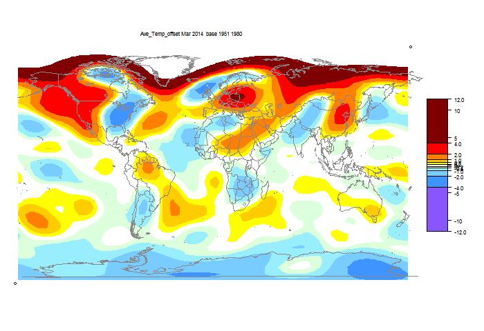
It was again cold in N America, but the spectacular cold spot was in central Africa. This may be an artefact (Update - error in GHCN, see above). Below is the map of the 4255 stations reporting to date. That is a fair total, but as the map shows, reports from central Africa are sparse. The natural suspicion is that I've pushed the resolution too far, but the cold spot shows at lower resolution. And I've used the revised method to recalculate previous months, with good results. We'll see what GISS says.

It was very warm in Europe and northern Asia.
Update 12 Apr: I've had to modify the plot (slightly) because the new SH routine wasn't setting the anomaly base correctly. Again, the global average is unaffected.



Update: Another apparent GHCN error. The station of NORD ADS, 81°N in Greenland, is shown with a monthly mean of 4.3°C. It's normally about -30 in March. I checked the CLIMAT forms, but OGIMET says Greenland hasn't submitted any in March.

Active viewer for Neukom et al proxies

A current paper in Nature from a long list of authors, including Neukom, Gergis and Karoly, on Southern Hemisphere proxies, is attracting attention. It's emphasis is on inter-hemispheric comparisons. The paper is here, the extensive SI here, and the data here. A press release is here.

There are critical posts at WUWT (here and here) and at Climate Audit.

So far I don't have an opinion on the study itself. But as with previous studies by Marcott et al and Pages2K, I have posted an active viewer, which gives easy access to plots and metadata. It's below the jump.

Update: I've added a choice of range. You can click on 2000 years to see the full range, or 400 years to see post-1600 on an expanded scale.






The methods are as for the Marcott viewer. The spaghetti curves are colored as their labels; since the proxies are ordered longest first, this creates a rainbow pattern. The annual data (2000 years) is very noisy, so I smoothed with a 10-year boxcar filter.

One of the tedious tasks here was getting a formatted table from the pdf Table 5 in the SI. I have put up a csv file of that table here.

At some stage I'll do a composite viewer for Marcott, Pages2K and Neukom.

There was a slight discrepancy between the order of proxies in Table 5 and the order of columns in the data. I've reset the Table 5 order to mtch.

WebGL code: shaded grids and maps

In a previous post, I described a generic specification for a WebGL representation of continuum data on a spherical Earth that you can rotate like Google Earth. Examples were cited. The idea was to separate out the task of geometry specification from the nuts and bolts of WebGL (which were hidden). But you still had to specify the geometry.

In this post, I want to simplify three common tasks:

• Drawing a shaded plot of gridded data.
• Specifying a palette (there's a default for grid shading).
• Adding a world map (just coast outlines)

It's reduced to the extent where you have to simply supply the gridded data as a comma separated list. In the example below, you can enter it by pasting into a text box, and press the "Plot New" button.

To enter a world coast outline map, just define an object with new type MAP. Nothing else required. I have also added a "title" attribute of an object. If supplied, the title will appear top left. It can be any HTML (including plain text).

So here is the new plot, showing GISS LOTI temperatures for January 2014. You can rotate to see the pattern of the Polar vortex. (Currently replaced with BEST trends). Below, I'll show the user code, and how you can add your own data.


The user JS file that I supply is:
function PxDat(p){
var C,M,p;
C=p[1];  //The grid
M=p[2]; M.type=MAP;
C.links=1; 
C.title="GISS LOTIJanuary 2014"
C.nodes=[1.42,1.42,...];
}
Easiest is object 2, the map. Just give the type.

For object 1, C (the grid), instead of node coordinates, in "nodes" I put the grid values, starting at (or near) the corner (90S,180W), and then in latitude bands. In "links" I give a single integer. This can be the number of horizontal cells, but if the cells are square, as usual, the digit 1 will do. Such grids usually are 2n x n, or maybe 2n x (n+1); the program will work out which. If it is neither of these, you should set .links to the number of grids in a latitude band.
You can still define a palette, as described previously. But for a grid, if you do not, the default is a rainbow palette with 256 colors, seen here.
You'll see that a color key is provided. This is centred at the mean of your data (as is the palette), and color spacing is finest there, dropping rather exponentially as you go away, so coarse for outlying values.

User data entry

You don't even have to do this much programming. If you have grid data as a comma separated list (from 90S, 180W), just paste it into the text box top right. There seems to be a limit of about 16000 characters. You can put a title in the box below. Then click "Plot New".
Here are some trivial examples, which still give some idea of how the shading is done. Try pasting in:
1,1,1,1,2,2,2,2
This is a 4x2 grid; you'll see uniform shading from bottom to top, Vary the numbers if you like. If the number of latitudes is even, it is treated as nodes at cell centres. So thete is a gap at each pole. It looks huge here, but of course is small in real grids. Now try:
-9,-9,-9,-9,3,-3,3,-3,9,9,9,9
This is a 4x3 array, and so the nodes are assumed at the corners of cells. So there's a row of nodes at each pole, and the cells show here as faces of an octahedron. The colors are mixed up a bit. Note how the color key adapts.

Where next?

Usually, providers such as GISS and HADCRUT supply gridded data on NCDF files. I use the R package "ncdf" to unravel there. Unfortunately, they usually pack a huge lot of data into these files; typically a century or so of months, for monthly data. Often there are several variables. Files can be tens, hundreds or thousands of megabytes. You'll need to extract a single grid, and even those can be big. JS input has to be text. Make sure to use rounding.
I have found good data rather hard to come by. Coarse grids like the GISS one above don't make good use of the much better WebGL resolution. Much better is something like the 1/4° SST data here. But there there is extra work to keep the land/sea boundary sharp. HYCOM has 1/12° data, but I'm finding the files just too big. I'd be glad of any suggestions.
If I can find interesting and regularly updated data, I'll rig up a scheme for updating and install a page like that for SST.

Code

I've updated the zip file from the previous post, here. The main JS is now in grid.js; the example here is grid0.js. But the HTML file is still Moygl.html. I think everything is backward compatible.

Paleo plotting - new draft climate plotter

In the previous post, in response to a challenge posed by Gavin at Real Climate for better ways of visualizing Phanerozoic climate data, I showed an interactive plot mechanism which could allow the user to easily vary the time scale in a single plot environment. The mechanics really come from the Moyhu climate plotter, and I've been meaning to work up a new version of that (and it's time to update with 2013 data).

A limitation in the V2 plotter was a restriction to annual data, and it generally covered the instrumental period. This reduced the data size, which is of some importance if all the data has to be downloaded. It also facilitates post processing - eg combining or smoothing series.

In V3 I've allowed all kinds of time data. I can overcome the size p[roblem by using XMLHTTPrequest, so only requested data is downloaded. And to allow the user to easily go from a century timescale to decade (for monthly data) or million years, I need to upgrade the user controls. Also to show monthly data, I will need an automatic updating system.

I'm posting a draft version here. It doesn't yet have request download, though download times are reasonable. And a lot of the post-processing doesn't yet work. Smoothing and regresion are patchy, and the calculate facility will probably go. But the basic plotting should work, and I'd be interested in comments, especially of datasets to include.

Adjustable plotting for multiscale global temperatures

This post relates to a challenge posed by Gavin at Real Climate, to better depict the long term history of temperature. Gavin linked to datasets ranging from instrumental (150 years) to Phanærozoic (540 M yrs). I have been experimenting with user-adjustable graphs (see also gallery). The big changes of scale are a challenge, but I thought it was worth a try. The current version is rough, but I'll put in more data, with selectable axes.

The graph initially shows the last 200 years or so, but with a temperature scale big enough to cover the whole period. You can adjust the scales as follows:

• Translation - by mouse dragging in the plot space. However, zero time (before 2014) is fixed to the origin.
  
• Temp scale - by dragging vertically in the space to the left of the y-axis.
  
• Time scale - this is the critical one. You can make fine adjustments by dragging below the x-axis. But faster is to click in the region with <...>, blue, bottom left. < shrinks the scale (longer times), and the response is proportional to how far you click from the centre (about double per <).
  

The data sets given by Gavin were:

Period	Reference	Data download
0-600 Mya	Veizer et al (2000), Royer et al (2004) (updated Royer (2014))	Veizer d180, Royer04 Temp, Royer14 CO2
0-65 Mya	Zachos et al (2008), Hansen et al (2010)	Zachos/Hansen
0-5.3 Mya	Lisiecki and Raymo (2005)	LR04 Stack
0-800 kya	EPICA Dome C	Temperature Reconstruction
0-125 kya	NGRIP/Antarctic analog?	NGRIP 50yr
0-12 kya	Marcott et al (2013)	MEA12 stack (xls)
0-2 kya	Mann et al (2008), Ljungqvist (2010)	MEA08 EIV, Ljungqvist10
1880-2013 CE	GISTEMP	GISTEMP LOTI
1850-2013 CE	HadCRUT4	HadCRUT4 Global annual average, Cowtan&Way (infilled)
1850-2013 CE	Berkeley Earth	Land+Ocean annual mean

I have currently done HadCRUT4, GISTEMP LOTI, Ljungqvist10, Marcott et al (2013), EPICA Dome C,Lisiecki and Raymo (2005), Zachos and Hansen, Veizer d180. L&R is d190O data, so I scaled to to match Z&H over the first 5 million years. Veizer is ocean bottom temperature, so I used a faint color - I'm currently just trying to get the scaling to work well. So here is the plot:
Update: As Gavin at RC noted, I had L&R upside (d18O). Fixed now.

Other imperfections

I haven't been careful with anomaly base - the data is as is. I tried adjusting sequentially by overlaps, but there is noise, and for the moment, I don't think it adds value.

I have smoothed and sampled opportunistically. Epica was smoothed by three boxcar filterings, length 5, and then sampling every fifth. Zachos was smoothed once and sampled every fifth. L&R was sampled. With smoothing, end regions were included unsmoothed.

I'll surely find more.

February GISS Temp down by 0.25°C

GISS showed a substantial decrease in February, going from 0.70°C to 0.45°C. This slightly exceeded the drop shown by TempLS, which in turn was somewhat greater than the drop shown by the satellite measures. GISS had shown a rise in January, while TempLS was steady.


In agreement with TempLS, the cold places were N America and Central Asia, with warmth in NE Europe. Here is the GISS map for Feb2014:


And here, with the same scale and color scheme, is the earlier TempLS map:

Previous Months

January 2014
December
November
October
September
August
July
June
May
April
March
February
January
December 2012
November
October
September
August
July
June
May
April
March
February
January
December 2011
November
October
September
August 2011

More data and plots