About a month ago, I posted on a proposed new scheme for reporting monthly averages with a mesh version of TempLS. The idea was to report continuously as data (land source GCHN) came in. I wondered how reliable the very early estimates might be. I was quite optimistic.
So, wouldn't you know, November is the first month in my experience when GHCN didn't keep to their regular schedule. Normally there are daily updates from month start, with the largest in the first day or two. But this month, nothing at all until the 8th. Sure enough, my program faithfully produced an average (0.589°C) based on SST alone; it's been told now not to do that again.
Anyway, the data has arrived, and is up on the latest data page. October (with GHCN) was 0.664°C; almost exactly the same as September, which was pretty warm. For once, there was little cold in N America, and W Europe was warm. The main cold spot was Russia/Kazakhstan.
Monday, November 10, 2014

Saturday, November 8, 2014
GCM's are models
I'd like to bring together some things I expound from time to time about GCM's and predictions. It's a response to why didn't GCMs predict the pause? Or why can't they get the temperature right in Alice Springs?
GCM's are actually models. Suppose you were designing the Titanic. You might make a scale model, which, with suitably scaled dimensions (Reynolds number etc) could be a good model indeed. It would respond to various forcings (propellor thrust, wind, wave motion) just like the real boat. You would test it with various scenarios. Hurricanes, maybe listing, maybe even icebergs. It can tell you many useful things. But it won't tell you whether the Titanic will hit an iceberg. It just doesn't have that sort of information.
So it is with GCM's. They too will tell you how the Earth's climate will respond to forcings. You can subject them to scenarios. But they won't predict weather. They aren't initialized to do that. And, famously, weather is chaotic. You can't actually predict it for very long from initial conditions. If models are doing their job, they will be chaotic too. You can't use them to solve an initial value problem.
GCM's are actually models. Suppose you were designing the Titanic. You might make a scale model, which, with suitably scaled dimensions (Reynolds number etc) could be a good model indeed. It would respond to various forcings (propellor thrust, wind, wave motion) just like the real boat. You would test it with various scenarios. Hurricanes, maybe listing, maybe even icebergs. It can tell you many useful things. But it won't tell you whether the Titanic will hit an iceberg. It just doesn't have that sort of information.
So it is with GCM's. They too will tell you how the Earth's climate will respond to forcings. You can subject them to scenarios. But they won't predict weather. They aren't initialized to do that. And, famously, weather is chaotic. You can't actually predict it for very long from initial conditions. If models are doing their job, they will be chaotic too. You can't use them to solve an initial value problem.
Friday, November 7, 2014
Climate blog index again
About a year ago, I described a Javascript exercise I began mid-2013, when Google Reader discontinued. I thought I might write my own RSS reader, with indexing capability. I found that feedly was a good replacement for Reader, so that didn't continue. However, I thought a more limited RSS index of climate blogs would be handy. A big motivation was just to have an index of my own comments (to avoid boring the public with repetition).
So I set up a page, and set my computer to reading the RSS outputs every hour. The good news is that that has happened more or less continuously. The bad news was that junk accumulated, and downloading was slow.
So I've done two new main things:
As with my blogroll, I've included blogs with broad readership; not necessarily the ones I recommend.
Here are some examples of selections:
Stoat, last two months (two months takes a few seconds to load)
My comments at WUWT, last two months
Posts by Bob Tisdale at WUWT in November
So I set up a page, and set my computer to reading the RSS outputs every hour. The good news is that that has happened more or less continuously. The bad news was that junk accumulated, and downloading was slow.
So I've done two new main things:
- Pruned the initial download. I had already reduced the initial offerring to just two days of comments. But I still downloaded details of all threads and commenters. More than half the commenters listed had only ever made one comment. They include of course various spammers, and typos. So I removed them, unless their comment was in the last month. I also divided the threads into current and dormant (no activity in two months). Current are downloaded at start; dormant can be added (button), or will come automatically if data more than two months ago is requested. It's faster, if not fast.
- I've added a facility where a string is shown that you can add to the URL to get it to go to the current state. That includes selected index items (commenter etc) and months. The main idea is that you can store a URL which will go straight to a list of your own comments over some period (remembering that each month takes a while to download). Examples below.
As with my blogroll, I've included blogs with broad readership; not necessarily the ones I recommend.
Here are some examples of selections:
Stoat, last two months (two months takes a few seconds to load)
My comments at WUWT, last two months
Posts by Bob Tisdale at WUWT in November
Wednesday, October 29, 2014
Calculating the environmental lapse rate
I have posted over the years on the mechanisms of the lapse rate - the vertical temperature gradient in the atmosphere. It started with one of my first posts on what if there were no GHE. My basic contention has been that lapse rates are a consequence of vertical air motions in a gravity field. Wind tends to drive the gradient toward the DALR - dry adiabatic lapse rate = -9.8 °K/km. Maintaining the gradient takes kinetic energy from the wind to operate a heat pump. The pump forces heat down, to make up for the flux transported up by the gradient. The pump effect is proportional to the difference between the actual lapse rate La and the DALR L. L is the stability limit, and a steeper gradient will convert the pump into an engine, with convective instability. This also pushes La (down) toward L.
I developed these ideas in posts here, here and here. But I have wondered about the role of infrared radiation (with GHGs), and why the actual gradient is usually below the DALR. The latter is often attributed to latent heat of water, and called the moist ALR. But that is only effective if there is actual phase change (usually condensation).
I now see how it works. The heat pump reduces entropy, proportionally to the energy it takes from the wind. The entropy can indeed be related to the gradient and the effective thermal conductivity; the largest component of that is a radiative mechanism. So the lapse rate rises to the maximum level that the wind energy can sustain, given the conductive leakage.
I'll write a simplified argument first. Consider a parcel of dry air, mass m, which rises vertically dist dz for a time, at ambient pressure P=Pa, starting at ambient temperature T=Ta. The motion is adiabatic, but it then comes to rest and exchanged heat with ambient.
The temperature inside the parcel drops at the same rate as the DALR, so the difference : d(T-Ta)/dz = -(L-La)
The density difference is proportional to this
d(ρ-ρa)/dz = -(L-La)*ρ/T
I'm ignoring second order terms in dz.
The net (negative) bouyancy force is
F = V g (ρ-ρa)
dF/dz = -V g (L-La)*ρ/T
The work done against bouyancy (power) is ? F dz = 1/2 V g (L-La)*ρ/T dz2
Note that this is independent of sign of z; the same work is done ascending as descending.
Because the temperature on arrival is different to ambient, heat has been transported. I could work out the flux, but it isn't very useful for macroscopic work. The reason is that not only is it signed, but separate motions convey heat over different segments, and there is no easy way of adding up. Instead, an appropriate scalar to compute is the entropy removed. Heat pumps do reduce entropy; that's why they require energy. Of course, entropy is created in providing that energy.
The simplest way to calculate entropy reduction is to note that the Helmholtz Free Energy U - TS (U=internal energy) is unchanged, because the motion is adiabatic. This means T dS and P dV (pressure volume work) are balanced. And P dV is from the buoyancy work. So:
T dS = -1/2 m g (L-La)*ρ/T dz2
where S is entropy
Assume there is a distribution of vertical velocity components v in a slice height dz. I can then re-express the work done as a power per unit volume: F v = 1/2 v.dx' g (L-La)*ρ/T
In Latex I'd use hats to indicate averages.
I've left in a dx' which was the old distance of rise, which determines the average temperature discrepancy between parcel and ambient. It's not obvious what it should now be. But I think the best estimate for now is the Prandtl mixing length. This is related to the turbulent viscosity, and in turn to the turbulent kinetic energy (per unit volume) TKE.
So now it gets a bit more handwavy, but the formula becomes
Average power/vol (taken from wind) ~ -g (L-La)/T * TKE
This follows through to the rate of entropy removal, which is
rate of entropy ~ -g (L-La)/T2 * TKE
(power divided by T)
Q = -k dT/dz
where k is a conductivity,
then the volume rate of creation of entropy is
dS/dt = -Q d(1/T) = -Q/T2dT/dz
= k La T-2
So what is k?. Molecular conductivity would contribute, but where GHG's are present the main part is infrared, which is transferred from warmer regions to cooler by absorption and re-emission. In the limit of high opacity, this follows a Fourier law in the Rosseland approximation
flux = 16 s G n2 T3 dT/dz
s Boltzmann's constant, G an optical parameter (see link), n refractive index. Three optical depths is often used as a rule of thumb for high opacity; we don't have that, but you can extend down by using fuzzy boundaries, where for eample there is a sink region where there is transmission direct to space.
Update: I forgot to say the main thing about G which is relevant here, which is that it is inversely proportional to absorptivity (with an offset). IOW, more GHG means less conductivity.
Update
I've made an error here. I assumed that the flow expansion was adiabatic. This is conventional, and relates to the time scale of the motion. But I've also assumed adiabatic for the entropy balance, and that is wrong. There is a through flux of energy, mainly as IR, as indicated. And that flux carries entropy with it. So the formula should be:
dS/dt = (k La - Q) T-2
where Q is the nett flow of heat. I'll correct below. It is significant, and may change the sign.
k La T-2 ~ g (L-La)/T2 * TKE
or
La - L ~ - (k La - Q)/g/TKE
Obviously, there is an unspecified constant of proportionality (with time units), which comes from the nature of turbulence. But I don't think it should vary greatly with, say, wind speed.
So what can we say about the discrepancy between environmental lapse rate La and theoretical DALR L (=g/cp)?
So what about moisture? That is what the difference between La and L is usually attributed to.
I think moisture is best accounted for within the DALR formulation itself. The DALR L is, again, L= -g/cp, where cp is the specific heat of the gas (air). But in the derivation, it is just the heat required to raise the temperature by 1 °C(OK, that is what sh means), and you could include the heat required to overcome phase change in that. That increases cp and brings down the lapse rate. The thing about the moist ALR is that water only has a big effect when it actually changes phase. That's a point in space and time. Otherwise moist air behaves much like dry. Of course, an environmental lapse rate is only measured aftre there has been much mixing
I developed these ideas in posts here, here and here. But I have wondered about the role of infrared radiation (with GHGs), and why the actual gradient is usually below the DALR. The latter is often attributed to latent heat of water, and called the moist ALR. But that is only effective if there is actual phase change (usually condensation).
I now see how it works. The heat pump reduces entropy, proportionally to the energy it takes from the wind. The entropy can indeed be related to the gradient and the effective thermal conductivity; the largest component of that is a radiative mechanism. So the lapse rate rises to the maximum level that the wind energy can sustain, given the conductive leakage.
I'll write a simplified argument first. Consider a parcel of dry air, mass m, which rises vertically dist dz for a time, at ambient pressure P=Pa, starting at ambient temperature T=Ta. The motion is adiabatic, but it then comes to rest and exchanged heat with ambient.
The temperature inside the parcel drops at the same rate as the DALR, so the difference : d(T-Ta)/dz = -(L-La)
The density difference is proportional to this
d(ρ-ρa)/dz = -(L-La)*ρ/T
I'm ignoring second order terms in dz.
The net (negative) bouyancy force is
F = V g (ρ-ρa)
dF/dz = -V g (L-La)*ρ/T
The work done against bouyancy (power) is ? F dz = 1/2 V g (L-La)*ρ/T dz2
Note that this is independent of sign of z; the same work is done ascending as descending.
Because the temperature on arrival is different to ambient, heat has been transported. I could work out the flux, but it isn't very useful for macroscopic work. The reason is that not only is it signed, but separate motions convey heat over different segments, and there is no easy way of adding up. Instead, an appropriate scalar to compute is the entropy removed. Heat pumps do reduce entropy; that's why they require energy. Of course, entropy is created in providing that energy.
The simplest way to calculate entropy reduction is to note that the Helmholtz Free Energy U - TS (U=internal energy) is unchanged, because the motion is adiabatic. This means T dS and P dV (pressure volume work) are balanced. And P dV is from the buoyancy work. So:
T dS = -1/2 m g (L-La)*ρ/T dz2
where S is entropy
Going macro
I've shown the work done and entropy generated by a single movement. I'll try to relate that to a continuum. I've used a particular artificial example to link work done with entropy removed. In fact, turbulence typically consists of eddy motions.Assume there is a distribution of vertical velocity components v in a slice height dz. I can then re-express the work done as a power per unit volume: F v = 1/2 v.dx' g (L-La)*ρ/T
In Latex I'd use hats to indicate averages.
I've left in a dx' which was the old distance of rise, which determines the average temperature discrepancy between parcel and ambient. It's not obvious what it should now be. But I think the best estimate for now is the Prandtl mixing length. This is related to the turbulent viscosity, and in turn to the turbulent kinetic energy (per unit volume) TKE.
So now it gets a bit more handwavy, but the formula becomes
Average power/vol (taken from wind) ~ -g (L-La)/T * TKE
This follows through to the rate of entropy removal, which is
rate of entropy ~ -g (L-La)/T2 * TKE
(power divided by T)
Temperature gradient as a source of entropy
If you have a steady temperature gradient, and a consequent heat flux Q determined by Fourier's Law:Q = -k dT/dz
where k is a conductivity,
then the volume rate of creation of entropy is
dS/dt = -Q d(1/T) = -Q/T2dT/dz
= k La T-2
So what is k?. Molecular conductivity would contribute, but where GHG's are present the main part is infrared, which is transferred from warmer regions to cooler by absorption and re-emission. In the limit of high opacity, this follows a Fourier law in the Rosseland approximation
flux = 16 s G n2 T3 dT/dz
s Boltzmann's constant, G an optical parameter (see link), n refractive index. Three optical depths is often used as a rule of thumb for high opacity; we don't have that, but you can extend down by using fuzzy boundaries, where for eample there is a sink region where there is transmission direct to space.
Update: I forgot to say the main thing about G which is relevant here, which is that it is inversely proportional to absorptivity (with an offset). IOW, more GHG means less conductivity.
Update
I've made an error here. I assumed that the flow expansion was adiabatic. This is conventional, and relates to the time scale of the motion. But I've also assumed adiabatic for the entropy balance, and that is wrong. There is a through flux of energy, mainly as IR, as indicated. And that flux carries entropy with it. So the formula should be:
dS/dt = (k La - Q) T-2
where Q is the nett flow of heat. I'll correct below. It is significant, and may change the sign.
Balancing it all - lapse rate determined
Now we have an entropy source term and a sink term. In steady state entropy can't accumulate, so they balance:k La T-2 ~ g (L-La)/T2 * TKE
or
La - L ~ - (k La - Q)/g/TKE
Obviously, there is an unspecified constant of proportionality (with time units), which comes from the nature of turbulence. But I don't think it should vary greatly with, say, wind speed.
So what can we say about the discrepancy between environmental lapse rate La and theoretical DALR L (=g/cp)?
- Proportional to k, the conductivity. So if GHGs transport heat in response to the temperature gradient, as they do, the lapse rate diminishes, away from L. With no GHG's, there is much less to separate L and La. Not so clear - see above correction.
- Inversely proportional to TKE (depends on wind speed). So stronger wind brings the lapse rate closer to L
- Proportional to (La -Q/k).
So what about moisture? That is what the difference between La and L is usually attributed to.
I think moisture is best accounted for within the DALR formulation itself. The DALR L is, again, L= -g/cp, where cp is the specific heat of the gas (air). But in the derivation, it is just the heat required to raise the temperature by 1 °C(OK, that is what sh means), and you could include the heat required to overcome phase change in that. That increases cp and brings down the lapse rate. The thing about the moist ALR is that water only has a big effect when it actually changes phase. That's a point in space and time. Otherwise moist air behaves much like dry. Of course, an environmental lapse rate is only measured aftre there has been much mixing
Thursday, October 23, 2014
Checking ENSO forecasts
I few days ago I commented here on the latest NOAA ENSO advisory:
""ENSO-neutral conditions continue.*
Positive equatorial sea surface temperature (SST) anomalies continue across most of the Pacific Ocean.
El Niño is favored to begin in the next 1-2 months and last into the Northern Hemisphere spring 2015.*""
I repeated this at WUWT, and someone said, but they have been saying that all year. So I ran a check on ENSO predictions.
The NOAA Climate Prediction Center posts a monthly series of CDBs (Diagnostic Bulletins) here. They are full of graphs and useful information. They include compilations of ENSO predictions (Nino3.4), nicely graphed by IRI. I downloaded the plots for each month of 2014, and overlaid with the observed value from this file.
It's an active plot, so you can click through the months. The year started out with a dip, mostly unforeseen. This coincided with the global cool in February. There was then a underpredicted recovery, and since then there has been a tendency for the index to be below predictions, esp June and July.
CPC warns that only modest predictive skill is to be expected, and that is fortified by the spread in forecasts. The index does indeed seem to move beyond the predicted range rather easily. It's not always overpredicted, though.
Here is the active plot. Just click the top buttons to cycle through the 9 months. The thick black overlay line are the monthly observations.
You'll see some minor discrepancies at the start. I don't think this is bad graphing - I assume minor changes to Nino3.4 between the monthly report and now. It looks like maybe a scaling error, but I don't think it is. I should note that I'm plotting the monthly value, while the foecasts are for three minth averages. I wanted to match the initial, which is one month. But Nino3.4 does not have much monthly noise, so I don't think averages would look much different.
""ENSO-neutral conditions continue.*
Positive equatorial sea surface temperature (SST) anomalies continue across most of the Pacific Ocean.
El Niño is favored to begin in the next 1-2 months and last into the Northern Hemisphere spring 2015.*""
I repeated this at WUWT, and someone said, but they have been saying that all year. So I ran a check on ENSO predictions.
The NOAA Climate Prediction Center posts a monthly series of CDBs (Diagnostic Bulletins) here. They are full of graphs and useful information. They include compilations of ENSO predictions (Nino3.4), nicely graphed by IRI. I downloaded the plots for each month of 2014, and overlaid with the observed value from this file.
It's an active plot, so you can click through the months. The year started out with a dip, mostly unforeseen. This coincided with the global cool in February. There was then a underpredicted recovery, and since then there has been a tendency for the index to be below predictions, esp June and July.
CPC warns that only modest predictive skill is to be expected, and that is fortified by the spread in forecasts. The index does indeed seem to move beyond the predicted range rather easily. It's not always overpredicted, though.
Here is the active plot. Just click the top buttons to cycle through the 9 months. The thick black overlay line are the monthly observations.
You'll see some minor discrepancies at the start. I don't think this is bad graphing - I assume minor changes to Nino3.4 between the monthly report and now. It looks like maybe a scaling error, but I don't think it is. I should note that I'm plotting the monthly value, while the foecasts are for three minth averages. I wanted to match the initial, which is one month. But Nino3.4 does not have much monthly noise, so I don't think averages would look much different.
Monday, October 20, 2014
More "pause" trend datasets.
In two recent posts (here and here), I have shown with some major indices how trends, measures from some variable time over the last two decades and now, have been rising. This is partly due to recent warmth, and partly to the shifting effect (on trend) of past events, as time passes.
This has significance for talk of a pause in warming. People like to catalogue past periods of zero or negative trend. A senior British politician recently referred to "18 years without warming". That echoes Lord Monckton's persistent posts about MSU-RSS, which does have, of all indices, by far the lowest trends over the period.
Here I want to show results about other indices. Cowtan and Way showed that over this period, the trend in Hadcrut was biased low because of non-coverage of Arctic warming. I believe that TempLS with mesh weighting would also account properly for Arctic trend, and this would be a good way to compare the two, and see the effect of full interpolation. I expected GISS to behave similarly; it does to a limited extent.
So a new active plot is below the jump. You can rotate between datasets and months separately. There is also a swap facility so you can compare the images. And I have individual discussion of interpolation data vs grid data groups.
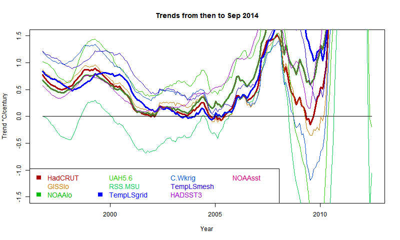
Here is the main plot. Buttons to rotate months and datasets. Emphasised set is in thicker black, on the legend too. (For some reason, NOAA emphasises as red). There is a reserved group of images for which the swap buttons work. It's initially empty, and you need at least two. In non-swap mode, click push to add the current image. In swap mode, click pop to remove the currently visible from the set.
General comments much as before. There is a big contrast between satellite indices MSU-RSS (long pause) and UAH (short). Trends are rising as the months of 2014 progress. I'm extrapolating to November assuming continuation of current weather, as described in previous posts. Trends are generally rising, which means it is getting harder to find long periods of non-positive trend ("pause").
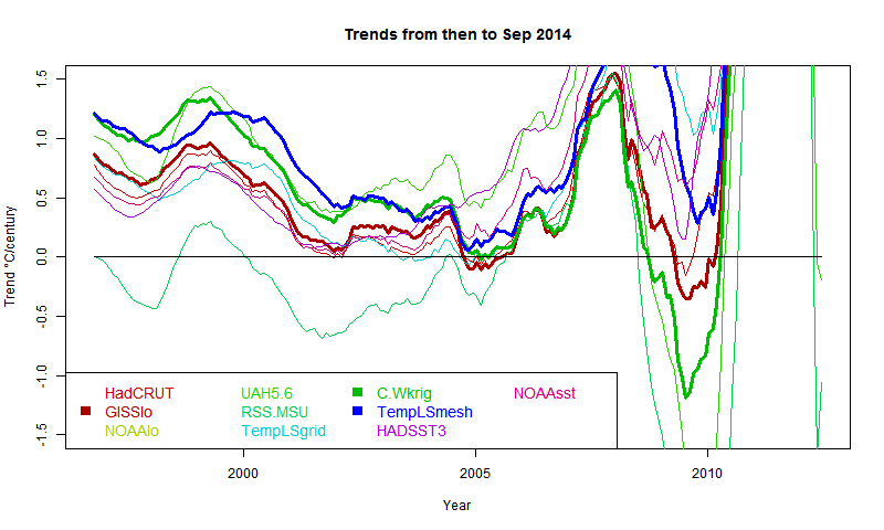
It shows C&W and TempLS tracking fairly closely from 1997 to 2008, with GISS generally a bit below.
This has significance for talk of a pause in warming. People like to catalogue past periods of zero or negative trend. A senior British politician recently referred to "18 years without warming". That echoes Lord Monckton's persistent posts about MSU-RSS, which does have, of all indices, by far the lowest trends over the period.
Here I want to show results about other indices. Cowtan and Way showed that over this period, the trend in Hadcrut was biased low because of non-coverage of Arctic warming. I believe that TempLS with mesh weighting would also account properly for Arctic trend, and this would be a good way to compare the two, and see the effect of full interpolation. I expected GISS to behave similarly; it does to a limited extent.
So a new active plot is below the jump. You can rotate between datasets and months separately. There is also a swap facility so you can compare the images. And I have individual discussion of interpolation data vs grid data groups.
Here is the main plot. Buttons to rotate months and datasets. Emphasised set is in thicker black, on the legend too. (For some reason, NOAA emphasises as red). There is a reserved group of images for which the swap buttons work. It's initially empty, and you need at least two. In non-swap mode, click push to add the current image. In swap mode, click pop to remove the currently visible from the set.
| Data | Month | Swap |
General comments much as before. There is a big contrast between satellite indices MSU-RSS (long pause) and UAH (short). Trends are rising as the months of 2014 progress. I'm extrapolating to November assuming continuation of current weather, as described in previous posts. Trends are generally rising, which means it is getting harder to find long periods of non-positive trend ("pause").
Interpolation groups
As Cowtan and Way found, whether or not you see a pause depends a lot on whether you account for Arctic warming. TempLS typifies this - the grid version, like HADCRUT, effectively assigns to empty cells (of which Arctic has many) global average behaviour, missing the warming. TempLS mesh has full interpolation, like the kriging version of Cowtan and Way. So here is the comparison plot, with C&W, TempLS and GISS in dark colors:It shows C&W and TempLS tracking fairly closely from 1997 to 2008, with GISS generally a bit below.
Grid surface data
And here for comparison are HADCRUT, NOAA Land/Ocean and TempLS grid. I expect these to be fairly similar. TempLS and NOAA have been very close lately, but over this longer range, TempLS is closer to HADCRUT.External sources
| HadCRUT 4 land/sea temp anomaly |
| GISS land/sea temp anomaly |
| NOAA land/sea temp anomaly |
| UAH lower trop anomaly |
| RSS-MSU Lower trop anomaly |
| Cowtan/Way Had4 Kriging |
| HADSST3 |
| NOAA sea temp anomaly |
Sunday, October 19, 2014
Tails of the Pause.
I've been writing lately about matters which, I'm sorry to say, lack scientific gravity. One is the possible record warm 2014, and the other is the tailing of the Pause, as measured by periods of negative trend. My excuse is, people do talk about them, and there is interesting arithmetic which I can illustrate.
In my "pause" posts, I showed plots of trend of global temperature to present, plotted for periods shown on the x-axis, with trend shown at the starting point. A "pause" starts when, for some index, the axis is first crossed from pos to neg. The plots were active, and you could see the curves rising steadily over recent months. This meant the start of the pause moves forward, with eventual jumps where a previous excursion below the line no longer makes it.
Here is the recent active (buttons) plot to show that effect:
In this post, I'll quantify the rate of motion, and describe how much cooling would be required to reverse the trend. The effect of a new month's reading depends on its status as a residual relative to the regression line for the period - ie is it above or below the line, and by how much. But one reading is a different residual for each such period. I plot the present month as a residual, again referred to the start year, and also plot the rate of change of trend produced by the current (August) temperatures.
Note that y occurs only in integrals (which are from 0 to x), so when we differentiate β, no need to differentiate y. So, after some calculus algebra,
dβ/dx = (6/x^2)(y - y0 - βx/2)
where y0 is the mean over the period. Since the regression passes through this mean midway, the last part of this is the end residual.
ie dβ/dx = (6/x^2) * residual
That gives the factor that determines the rate.
So my first plot is the rate of rise, shown as a 3 month incrementwith August trends dotted
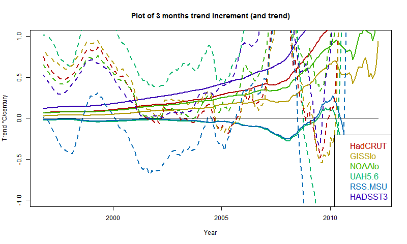
The satellite measures aren't going to move much without substantial warming. However, UAH is already high, RSS is low. Of the surface indices, HADSST3 is rising fast, GISS relatively slowly. However, three months of current warmth makes a big difference to the pause.
And here is the plot of residuals of August temp relative to past regressions:
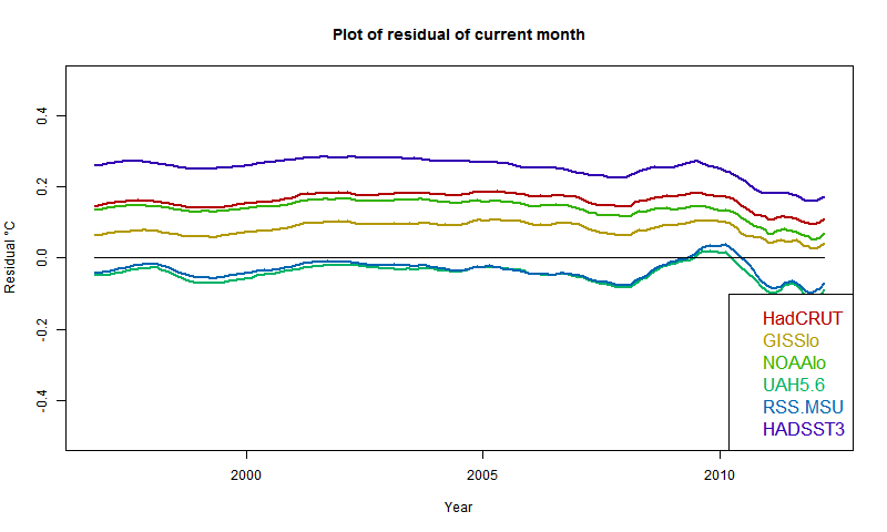
It confirms that UAH and RSS are near zero, so continuation of present temps won't change anything (though UAH warmed in Sept). Otherwise, GISS has the lowest residual, but positive everywhere; HADSST3 the highest. This of course partly reflects past coolness of HADSST3.
So if temperatures drop about 0.07°C from August, the rise for GISS would pause (but GISS rose in September). It would take a drop of more than 0.2°C for HADSST3.
In my "pause" posts, I showed plots of trend of global temperature to present, plotted for periods shown on the x-axis, with trend shown at the starting point. A "pause" starts when, for some index, the axis is first crossed from pos to neg. The plots were active, and you could see the curves rising steadily over recent months. This meant the start of the pause moves forward, with eventual jumps where a previous excursion below the line no longer makes it.
Here is the recent active (buttons) plot to show that effect:
In this post, I'll quantify the rate of motion, and describe how much cooling would be required to reverse the trend. The effect of a new month's reading depends on its status as a residual relative to the regression line for the period - ie is it above or below the line, and by how much. But one reading is a different residual for each such period. I plot the present month as a residual, again referred to the start year, and also plot the rate of change of trend produced by the current (August) temperatures.
Rate of change
This is more simply described with a continuum version. A time period runs from 0 to x, with readings y. If x increases, what is the change to trend β. The continuum formula is β = (x ∫ xy dx - x*x/2 ∫ y dx)/(x^4/12)Note that y occurs only in integrals (which are from 0 to x), so when we differentiate β, no need to differentiate y. So, after some calculus algebra,
dβ/dx = (6/x^2)(y - y0 - βx/2)
where y0 is the mean over the period. Since the regression passes through this mean midway, the last part of this is the end residual.
ie dβ/dx = (6/x^2) * residual
That gives the factor that determines the rate.
So my first plot is the rate of rise, shown as a 3 month incrementwith August trends dotted
The satellite measures aren't going to move much without substantial warming. However, UAH is already high, RSS is low. Of the surface indices, HADSST3 is rising fast, GISS relatively slowly. However, three months of current warmth makes a big difference to the pause.
And here is the plot of residuals of August temp relative to past regressions:
It confirms that UAH and RSS are near zero, so continuation of present temps won't change anything (though UAH warmed in Sept). Otherwise, GISS has the lowest residual, but positive everywhere; HADSST3 the highest. This of course partly reflects past coolness of HADSST3.
So if temperatures drop about 0.07°C from August, the rise for GISS would pause (but GISS rose in September). It would take a drop of more than 0.2°C for HADSST3.
Subscribe to:
Posts (Atom)


 Posts

