Friday, October 17, 2014

Record warmth in 2014?

Not according to the satellite measures; they are showing quite a cool year so far. But surface measures, apparently propelled by SST, have been consistently high since March, and a record for calendar 2014 looks possible.

In August 2010, I showed a plot of the progress of the cumulative monthly anomaly sums, which will reach the final sum that determines the year average. 2010 did turn out to be the hottest year in many indices. It was different in that the El Nino was late 2009/10, so late 2010 was cooling. At this stage 2014 seems to be warming.

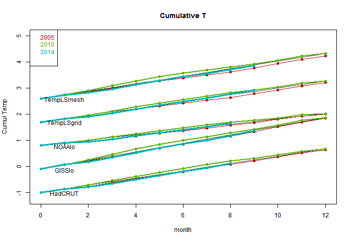
So I started to repeat that 2010-style plot, which is below the jump. It didn't work as well; the variation doesn't much show. But it puts the thing calculated in context - a cumulative sum that, if it exceeds 2010 at year end, will set a record. I've shown the progress of 2005 (a previous record), 2010 and 2014, with a line showing the 2010 average rate. The plots are spaced with an arbitrary offset.

But, more effectively, there is then an active plot with the average 2010 trend subtracted. The variation is clearer. The key thing is not so much whether the current total is above the line, but how it is trending, which is a measure of current warmth.

So here is the first plot. The TempLS measures were described in this recent thread. The absolute slope is an artefact of the anomaly base - GISS is earliest.


And here is the active plot with the 2010 average subtracted. Use the buttons to click through.


NOAA and TempLS grid are already above the line and heading up. Top candidates for a record. HADCRUT looks likely too. GISS and TempLS mesh only need a reasonable continuation of current warmth to end up positive (record). The slope is positive only when a month exceeds the average for 2010, so it doesn't take much cooling to turn down. We'll see.


Thursday, October 16, 2014

QC for TempLS


I plan to do more with TempLS (see last post) so I want a stable quality control (data) scheme. GHCN unadjusted is a document of record, and there is weird stuff in there which it seems they don't like to touch. I've noted current examples earlier in the year. So I did a survey of the data since 1850. Here is R's summary of the monthly averages:


Min. 1st Qu. Median Mean 3rd Qu. Max. NA's
-87.0 6.6 15.9 14.5 24.1 154.41166444

That's out of 10349232 months (of years with some data). Yes, the max is 154.4°C. There were 28 months with a min/max (not max) average >50°C.

To be fair, they use flags, and these oddities seem to be mostly where a decimal point slipped in the originating data. But they are big enough to have effects, so I have been using my own QC. On first look, I found the GHCN flags numerous and unhelpful, so I used a scheme where I checked with the adjusted file. This seemed to weed out the problem points without replacement. However, it excluded a lot of other points, so I allowed those if within 3°C of the appropriate mean.

I did that for the last five years of data and it worked well enough. But then I thought I should try for the whole record. I worked out how to extract the QC flags; here is a table of their occurrence:

DLMOSW
5511098112464722390454481981

The first column is no flag. QC flags aren't that common, about 0.24% of the total. The letters mean, according to the readme:
  • D - apparent duplicate
  • L - isolated
  • M - manual
  • O - outlier (>5 sd)
  • S - not so outlier (>2.5 sd), but no nearby data in agreement
  • W - seems to be last month

O and S are the big ones, and as expected, the very high ones are flagged O.

So I decided to just omit all flagged data. In future, I'll do that to all GHCN unadjusted before use.

If you've been watching the latest data over the last day, you'll have seen me experimenting. I think it is stable now.


Monday, October 13, 2014

A catch-up on TempLS

I've been writing a lot about TempLS (my global temperature index) recently, and realizing that I don't have a unique reference that explains exactly what it is and what has recently been happening to it.

TempLS dates back to a period in early 2010 when there was a flurry of amateur efforts to replicate the monthly global surface temperature indices from the major producers (which some thought suspect). This post by Zeke (with links to earlier) gives an overview. Jeff Id and Romanm started it with a reconstruction that used a least squares method for aggregating a single cell, yielding offsets rather than requiring a fixed anomaly period. I thought that could be applied to the whole recon.

So I developed TempLS, which was basically a big OLS regression, based on GHCN unadjusted station monthly averages. It was quick to run, and I incorporated choice mechanisms which made it easy to calculate regional or special (eg rural, airport) averages. A rather complete summary of this stage of development is here. An important feature was the incorporation of SST data. This comes gridded, often 5°x5°, and so I simply entered these as stations.

I made a point of using unadjusted GHCN, because there were many claims that warming was an artefact of adjustment. I have myself no objections to adjustment, though I did show that it makes relatively little difference to the index.

TempLS combines weighted regression with spatial integration, much as BEST did later. It weighted initially by the inverse of grid density, estimated by stations/cell in a 5°x5° grid. I posted at one stage a very simple version for incorporation in Steven Mosher's RGHCNv3. You can regard this weighting as that which a spatial integration formula woud provide, with each grid estimated by its station average anomaly, or equivalently, each function value (observed average) assigned an area equal to its share of the cell.

Version 2 in August 2010 generalised the idea of regression, so that spatial variation (among others) could be included (and maps produced). The math basis was set out here.

Meanwhile I was experimenting with other kinds of weighting. The problem with cell averages, which I now cell grid weighting, is that many cells have no stations. These would be best represented by local data, but the weight that can be assigned is limited to one cell area, and near the poles, where there is a lot of sparseness, the cell areas actually diminish, so such regions are under-represented. In early 2011, I did a series on Antarctica (final and links). This developed various forms of mesh-based weighting. This means that every point is estimated based on local data. I tinkered with Voronoi tessellation, but have now settled with weighting that assigns to each node a weight equal to a third of the area of the triangles (from a convex hull, which provides an irregular triangular mesh) which touch it. This is equivalent to a finite element piecewise linear integration formula.

An interesting exercise, which I started in early days, is to see if some very small subset (60) of stations can give a reasonable world estimate. This is the latest in that series, with links back.

Version 2.1, which incorporates some revised verion, is described here. This is the last formal release with code.

Meanwhile, in July 2011 I started a regular cycle of posting a monthly average estimate, based on GHCN and SST - initially HADSST2, but I soon switched to ERSST. I tried to make sure to post ahead of the majors, so that a prediction record could be established. I then published a comparison with the GISS result for the month. A list of links to those posts is given here; each has a list to its preceding TempLS post. I also included the TempLS results with the other indices on my latest data page, and in the graphical comparisons there.

I posted a review of the comparison of TempLS with other indices in December 2012. It was clearly in the mainstream, closest to NOAA and HADCRUT. More recently, I posted a mini-review noting that the closeness to NOAA had become more pronounced.

I had thought of switching to mesh weighting for regular monthly, but was deterred by the hour+ it takes to do 1200 meshes to cover a century. But you don't need a new mesh each month; most historic months change the population of stations very rarely. So with a scheme of stored weights and detecting changes, I can do it, and I think I should. I expect the results to be now closer to GISS. I also expect that the results will compare well with the revision of Cowtan and Way; I'll post on that soon.

Appendix/Update

Carrick asked for more details on the use of meshes in integration. The FEM idea of integration is that you build up an interpolation which is exact at each node, and takes some polynomial form in between. They do it with basis functions, but we don't need to deal with that here. Just imagine that you have a linear interpolation on each triangle. They will match at the edges.

On the integration, first I'll formalize the trapezoid analogy. If you have two points z1,z2, with function values f1,f2, then the area of the trapezoid on the graph for the linear interpolation is (z2-z1)*(f1+f2)/2. Base length times mean height.

The corresponding formula in 3D is volume = base area * (f1+f2+f3)/3.

To prove it, let the linear approx be f=a.z+c. (a,z,vecs, . scalar product). Then f1 = a.z1+c etc.

To save writing determinants I'll invoke what I hope is a familiar proposition. The centroid z0=(z1+z2+z3)/3 is also the center of mass. ie ∫ z dA = z0 A, where A is the area of triangle (z1,z2,z3).

So ∫ f dA = a . ∫ z dA + ∫ c dA = (a . z0 + c)*A
= A * Σ_i ( a . z_i + c)/3 = A * (f1+f2+f3)/3

Now when you collect all the formulae for each triangle (FEM assembly), you get a big sum in which each node value f_i is multiplied by 1/3 of the sum of all the areas of triangles of which it is a node. That is the weighting I use (actually, no need to divide by 3).
<
Sunday, October 12, 2014

GISS September 0.77°C, up by 0.08°C

This my first report in the new style, where I record details of both mesh-weighted and traditional grid-weighted TempLS, along with the latest GISS. It is part-mechanical, but I annotate. TempLS numbers on the latest data page are constantly updated, but the monthly reports here won't change.

So the headline is, a very warm month. I think in GISS at least, 2014 may well be a record year. TempLS mesh showed a similar rise; TempLS grid dropped slightly. I expect the mesh version to more closely follow GISS, and the grid version to continue tracking NOAA. My next post will probably be an updated explanation of TempLS.

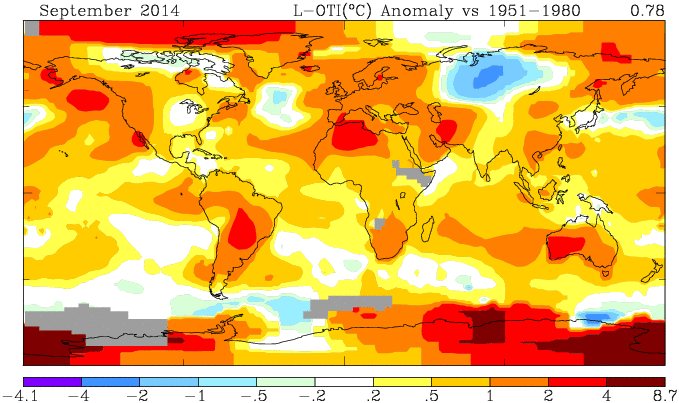
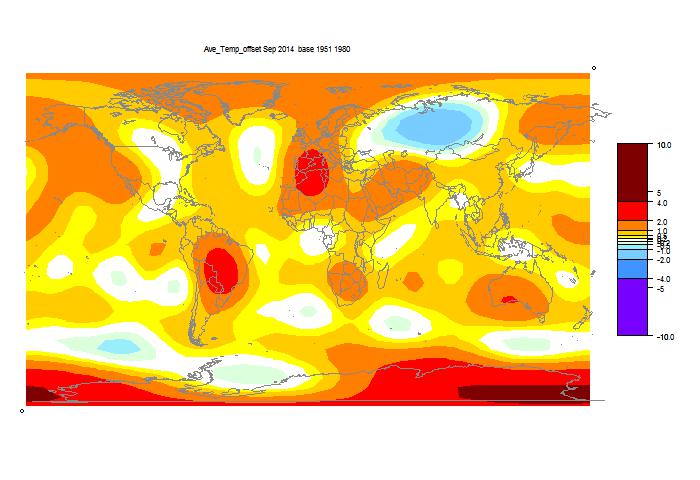
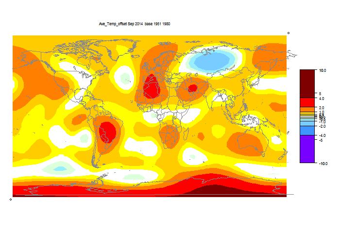
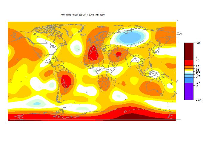
I've given both TempLS maps below. You can see again that TempLS mesh is closer to GISS than grid.

Comparison of GISS and TempLS, Sun 12 Oct 2014


Anomaly °CAprMayJunJulAugSep
GISS0.710.780.610.520.690.77
TempLS mesh0.6410.6690.580.4770.6270.673
TempLS grid0.6120.6070.580.5150.6150.598
Anomaly base years: GISS 1951-80, TempLS 1961-90.

Here is the GISS map


Here is the spherical harmonics based plot, mesh weighting


Here is the spherical harmonics based plot, grid weighting


List of past reports

New ideas on TempLS reporting - mesh

For over three years now, I've been running my least squares based GMST index TempLS each month and reporting the results, with a second post comparing with GISS. See here and here for last August. The second has past links. I did a mini-review here recently, and there is a new summary of TempLS here.

I'm planning a change. For some time, I've believed that using mesh based weighting (see here and here, for example) is better than what I call grid-based weighting, where observations are weighted on a cell-based density estimate. I was deterred from changing because the mesh generation took a long time, but I've fixed that. I'll persist with the grid model because as I noted, it has uncanny agreement with NOAA, and also tracks HADCRUT well. But I think that it also has the faults of those, in dealing with empty cells. For TempLS it takes the form that stations in empty areas have a capped weight based on the size on one cell, which in the Arctic can be small.

The data cycle goes like this. ERSST posts a preliminary on about 3rd or 4th of month. It's actually complete, and the numbers are little different when updated in late month. GHCN starts the month with a rush of numbers from places with efficient electronic systems, and then stuff trickles in fairly slowly. Lately GHCN (unadjusted) has had early gyrations too. But notwithstanding, I think it is meaningful to to a mesh baed calc as soon as the SST comes in. Mesh is more robust to missing.

I've now posted an automatic report on the latest data page. It shows the current mesh-based report, with maps of temperatures and of reporting stations. I think I can maintain this, reporting with every new GHCN (most days). It would flip to the new month when the SST is posted. Obviously, early figures would be subject to change.

This would supersede my first monthly report on the grid results. I'd still publish the GISS comparison, and record the grid and mesh TempLS results there.

Update. GISS has produced a map for September, and it says the Sept temperature is 0.78°C, up from 0.70°C in August. This tracks the mesh TempLS rise from 0.628°C to 0.673°C (grid TempLS went down slightly). I expect that mesh TempLS will follow GISS more closely. I'll post the GISS comparison soon. The new number is not yet on their datafile. It's getting warm.

Saturday, October 11, 2014

TempLS global temp down 0.017°C in September

TempLS cooled slightly; from 0.615°C (July) to 0.598°C. That is still quite high, following the previous rise of about 0.1°C. Anomaly base is 1961-90. For the satellite indices, MSU rose slightly, and UAH quite a lot, from 0.19°C to 0.29°C.

GHCN had ups and downs lately. For a few days, almost all the land data for August except USA vanished. In Sept, China data has only just arrived. I think everything is OK now.
Here is the spherical harmonics plot:


Warm in Antarctica, around Paraguay and Algeria. Cool in mid-Russia.
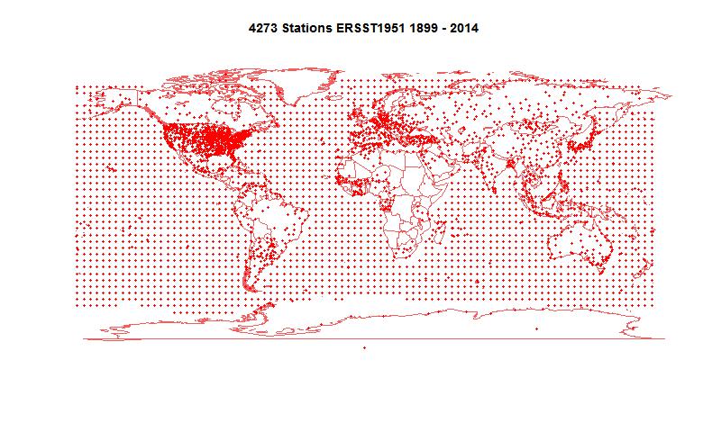
4273 stations reported. Here is the map:


Thursday, October 9, 2014

Portal for GHCN Daily

Many people are aware of GHCN Monthly. This is the large compilation of station monthly averages used for making global indices. I posted a portal here. Fewer know about GHCN daily, which is a very large compilation of daily records. Partly because of its size, it is less accessible. Each station record is in a separate file, and even listing the "all" directory takes a long time.

It is far less organized than GHCN Monthly. Many records are very short and incomplete. There is a mixture of TMAX, TMIN, precipitation, and various things like snow. Not easy. It is, however, for those who like that sort of thing, unadjusted. Very raw data.

So I've organised some links. I've split into US1, USC, Australia, Canada and others. US1 seems to have little or no temp data. USC is basically the Co-op network. The Australia record is huge, but a lot is rainfall. Canada is also large. So I've broken down those by states, and other countries are in the "World" list. Even there, some very significant countries are in the "Other" group at the end. Coverage is very uneven.

I've marked the files that have temp data (well, TMAX) with the years of record. As I mentioned, these can be short, and full of gaps at that. Entries without years probably don't have temperature. On the "Other" list, I've also marked where each country block begins.

So it's below the jump. You request by selecting from one of the menus. Clicking on a link will make the actual record pop up in a separate window or tab. I'm planning to create a permanent page for the various portals.

Update: I've added buttons that with Chrome will force the selection to take effect.


US1