Tuesday, May 17, 2011

Chladni patterns

At Climate Audit, Steve McIntyre has been frequently writing about Chladni patterns in connected with principal components of autocorrelated data. He developed it for the Steig paper, and was disappointed when J Climate wouldn't allow its inclusion in the response. And he's recently claimed an appearance in another paper.

Chladni patterns are modes of oscillation, originally of a vibrating plate. Now people more often think of a drum membrane, which is a slightly different wave equation, but the idea, and patterns, are similar.

I must admit that I hadn't heard of Chladni before Hans Erren drew attention to them in Steve's first post. Some interesting history there. But I am familiar with the modes in question.

Steve thinks that if a Chladni pattern emerges, that somehow means that the result is showing that rather than the information about the climate pattern being sought, so the information content is reduced. I don't agree - there are reasons why the patterns arise, and they are just as informative in PCA as they are in wave studies. I'll try to show why.

Warning - mathematics (and \(\LaTeX\)) after the jump.


Resonance and wave equations

Resonance is familiar with acoustics. If you speak in the open air, your voice propagates away in all directions, attenuating without reflection or selective amplification. If you stand in a partly enclosed cavity, your voice is slightly louder in certain frequency bands. In a totally enclosed bare room, you hear a characteristic booming response - some frequencies are much louder.

These are the ones that excite a resonant mode, in which the air oscillates, but the normal velocity at the boundary is zero. A 3D version of the modes of a vibrating stretched string, which has zero velocity at its ends.

The essential requirement is that the wave energy must be confined but not dissipated. That is why the resonance improves in deeper cavities, for example.

The wave equation for pressure, say, is (with c=speed of sound) $$\nabla^2 p = \frac{1}{c^2}\frac{\partial^2 p}{\partial t^2}$$ If you substitute a resonant mode \(p=P \sin(\omega t)\), then the equation is $$\nabla^2 P = -(\frac{\omega}{c})^2 P$$ P is the resonant mode, and so is an eigenvector of the Laplacian \(\nabla^2\). The resonant frequencies correspond to the eigenvalues.

For Chladni's plate the wave equation is more complicated, but the principle is the same.

Spatial autocorrelation.

Steve McI also described the simple Toeplitz autocorrelation coefficient matrix that you get in one dimension for a spatial model. With N+1 equally spaced points, the coefficients can be assumed to be powers of r - the correlation of adjacent sites. The matrix is: $$R = \left(\begin{array}{ccccc} 1 & r & r^2 & \ldots & r^N\\ r & 1 & r & r^2 & \ldots \\ r^2 & r & 1 & r & \ldots \\ \ldots & \ldots & \ldots & \ldots & \ldots\\ r^N & \ldots & r^2 & r & 1 \end{array}\right) $$ The Toeplitz property is that all terms on each diagonal are the same. This correlation matrix has a simple inverse: $$R^{-1} = \left(\begin{array}{ccccc} q & -qr & 0 & \ldots & 0\\ -qr & 2q-1 & -qr & 0 & \ldots \\ 0 & -qr & 2q-1 & -qr & \ldots \\ \ldots & \ldots & \ldots & \ldots & \ldots\\ 0 & \ldots & 0 & -qr & q \end{array}\right),\quad q=\frac{1}{1-r^2} $$ Still a Toeplitz matrix, almost, but also banded - tridiagonal. The deviation from Toeplitz is at the top left and bottom right corner terms.

Relation to Laplacian and the wave equation

From the last equation, $$\begin{align} R^{-1} &= qr\left(\begin{array}{ccccc} 1/r & -1 & 0 & \ldots & 0\\ -1 & r+1/r & -1 & 0 & \ldots \\ 0 & -1 & r+1/r & -1 & \ldots \\ \ldots & \ldots & \ldots & \ldots & \ldots\\ 0 & \ldots & 0 & -1 & 1/r \end{array}\right) \\ &= qr\left(\begin{array}{ccccc} 1 & -1 & 0 & \ldots & 0\\ -1 & 2 & -1 & 0 & \ldots \\ 0 & -1 & 2 & -1 & \ldots \\ \ldots & \ldots & \ldots & \ldots & \ldots\\ 0 & \ldots & 0 & -1 & 1 \end{array}\right) + q(1-r)^2 \left(\begin{array}{ccccc} 1/(1+r^2) & 0 & 0 & \ldots & 0\\ 0 & 1 & 0 & 0 & \ldots \\ 0 & 0 & 1 & 0 & \ldots \\ \ldots & \ldots & \ldots & \ldots & \ldots\\ 0 & \ldots & 0 & 0 & 1/(1+r^2) \end{array}\right) \end{align} $$ If you remember finite differences, the first matrix is just the negative of the second difference operator, corresponding to the 1D Laplacian. And the second is almost a multiple of the identity, and is small if r is close to 1.

That's the key to the connection between Chladni patterns and the autocorrelation matrix R. The inverse of R and the Laplacian of the wave equation differ by close to a multiple of the identity, which means they have almost the same eigenvectors. And the eigenvectors of R and \(R^{-1}\) are the same. R is symmetric and positive definite.

Subtle differences

Well, an unsubtle difference is that Chladni oatterns are not 1D. But the same reasoning works - it's too messy to set out here.

The subtler difference is that the diagonal correction is not quite Toeplitz. That relates to the notion of boundary conditions for the wave equation, which is indeed critical for resonance.

At this stage I'll have to just arm-wave on that - it does in fact give the zero normal boundary condition, which is sufficient for resonance.

Conclusion

The same mathematics that gives Chladni for the wave equations gives similar eigenvectors for the spatially autocorrelated matrix. It isn't a spurious consequence. Consequently their appearance in, say, Steig et al 2009 doesn't mean that the PC's are "just Chladni" any more than they are just autocorrelation. Spatial autocorrelation is an essential part of the results, and the Chladni patterns reflect that.

I think that's enough heavy maths for now - I could later go more into the properties of Chladni patterns, and in particular into the implications for eigenvalue pairing (for PCs) which SM criticised in Steig et al. That would generate pretty pictures.

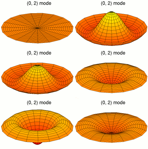
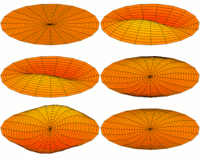
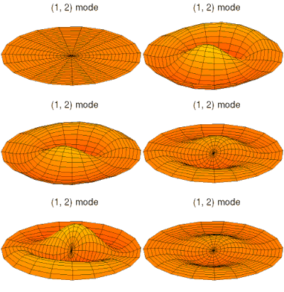
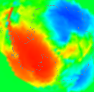
Meanwhile, I'll just relay these pictures of resonant modes from Wikipedia where more Chladni patterns on the disc and sphere can be found.


Latex now works here

I have implemented Latex (the MathJax version). It seems to work in comments too. You can just write normal Latex between these symbols(remove the _s)
  • \_(...\_) for inline
  • \_[...\_] or $_$...$_$ for display equations - note the doubled $'s
The next post should give this a workout.

The Woody Guthrie Award - Bart Verheggen


Last November, I was very pleased and flattered when ScienceofDoom chose Moyhu as the recipient of the Woody Guthrie award.

This award has an interesting history - it was initiated as a commendation of a "thinking blogger". The award was passed to SoD from Skeptical Science. I think both have been highly respected for their dedication to dispassionate analysis, and Moyhu has sought to live up to that.

I think Bart impressed all sides of the climate debate with his hosting of the very popular discussion on comparing temperature indices, which evolved into a debate about time series, unit roots and random walks. Strong views were expressed by well-informed commenters led by VS. Bart kept the discussion on track and constructive, with 2186 comments made. I think it is the best technical climate discussion I have seen.

But his blog isn't just technical - there is thoughtful, well-informed and inclusive discussion of policy as well. Bart always takes a broad view.

And there are brilliant cartoons as well.

I commend Bart's blog to readers, and I am very pleased to pass on the Award to him.


Here it is:
.


Thursday, April 14, 2011

Quiet time

Why is June hotter seen with GHCN V4 than V3 - and lots of active graphics.

This post is a follow-up to one a few days ago on differences seen calculating monthly global averages using TempLS and version 4 of GHCNrather than V3. It followed a post of Clive Best, who has a similar program, and was finding differences. I too found that June 2019 rose about 0.07°C while using GHCN V3 did not show a rise. I think overall differences are small, but I wanted to look at the underlying arithmetic.

So, as foreshadowed, I adapted my program to use its LOESS based calculation and graphics, in which I could calculate differences. But there was mission creep, as I found that being able to put disparate data on the same equally spaced grid made a lot of other things possible. So I showed also the effects of homogenisation. It does answer the question of why V4 made a difference this month, but there is a lot more to learn.

First let me tell the many uses of the main graphic, which is shown below. It is the familiar WebGL trackball Earth. You can drag it about and zoom. Click on the little map to quickly center at a chosen point. But importantly for this inquiry, you can control the content. The checkboxes top right let you switch on/off the display of V3 and V4 or SST nodes, or the shading (called "loess"), or even the map. And the radio buttons on the right give the choice of five data sets for June 2019, which are
  • Un V4-V3 which is the difference of TempLS anomalies using unadjusted GHCN data from V4 and V3.
  • Adj V4-V3 the corresponding difference using adjusted GHCN data (QCF, pairwise homogenised)
  • V4 Un - Adj the difference between unadjusted and adjusted data, for a V4 calculation
  • V4 Un - Adj same for V3
  • V4 Unadjusted just the TempLS anomalies using V4. It is the LOESS version of my regularly updated mesh plot.
So I'll show the plot here, with below an expanded discussion of what can be learnt from it.


Improved coverage in GHCN V4

This is shown most clearly if you switch off loess, and toggle the boxes controlling V3 and V4. The improvement of coverage is greater than I had thought, and as I will show is the basis for V3/V4 discrepancies.

The V3/V4 difference for June, and reasons.

One thing that surprised me was the coherence of the difference plots. The LOESS does some smoothing - you can estimate the effect by looking at the smudging around coastlines. The SST is the same between versions, so color in the sea means either islands or smoothed land. It fades basically exponentially, so color difference tends to exaggerate the spread. It's surprising because you would expect that station differences between V3 and v3 would be fairly random.

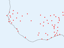
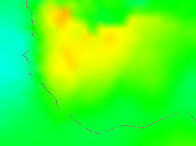
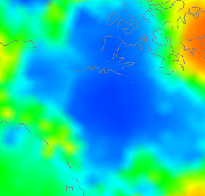
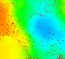
But only if both types are represented, and that is the key here. There is, for example, in Un V4-V3 a big warm patch around Senegal. I'll show also the station distribution and the anomalies:

V4-V3 differenceV4 stationsV4 anomaly

I haven't shown the V3 stations, because basically there aren't any (check the figure). So how did V3 cope? It used information from nearby, a lot of which was sea. V4 had much better coverage, so the region is predominantly represented by land. And as the third column choes, the land was warmer, by anomaly. Not a lot, but watch for the different color scales here. The apparent warmth in the first column is a much smaller temperature difference - the scales are about 4:1.

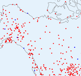
So here is where a discrepancy arises - an area which V4 covers much better, which happened to be warm that month. Here is an example going the other way in NW Canada:

V4-V3 differenceV3 and V4 stationsV4 anomaly

have shown the same tableau, but this time the centre plot shows V3 stations as well (in blue) since there are a few. But not many. Again what is happening is that the rather faint blue patch on the right, because it is picked up by V4 but hardly by V3, turns into a V4-V3 discrepancy on the left. One more case - Antarctica:

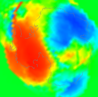
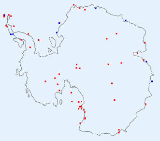
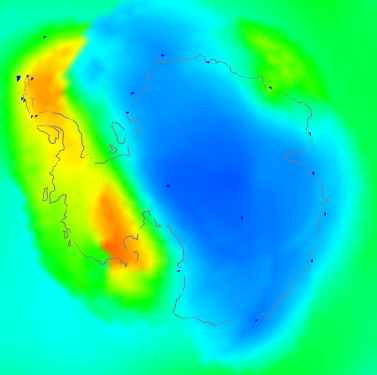
V4-V3 differenceV3 and V4 stationsV4 anomaly

This is a bit of both. It shows a discrepancy plot warm (ie high V4-V3) in the W, opposite in the East. The station plot shows a big increase in coverage in the interior, and also on the peninsula. And the right shows that the actual anomaly was also strongly divided between W and E. You might ask - why did the strong warmth in the East show a relatively small discrepancy? I think it is because although the V3 stations were sparser, they did give reasonable coverage around the coast of EA. So although the interior had to look far afield to infer temperatures, mostly it found land rather than sea.

So overall I think that is the cause. There are a few regions around the Earth where V4 has much better coverage. If these happen to align with anomaly patterns, those patterns will be reflected in the V4-V3 difference, and because there are only a few, from time to time they will align by chance.

I think this also explains the small persistent long term changes. As warming proceeds overall, it will more often happen that the anomaly patterns in V3-sparse areas with vary from SST on the warm side, producing a warm V4-V3 difference, which will accumulate.

What about adjusted data, whch seems to show a little more warming? I think it just fixes some aberrant cases which would reduce the effect in unadjusted data. Here is another tableau from Antarctica

Unadjusted V4-V3Adjusted V4-V3


The unadjusted had a number of blue spots along the Antarctic peninsula. Homogenisation identified some of these as biases that could be corrected. Whether right or wrong, the arithmetic result is of a discrepancy that integrates to a higher value, because of reduced noise.

To summarise, I think the reason is not that V3 stations were reporting temperatures different to V4; it is that in some regions they weren't reporting temperatures at all, and the discrepancies are a resulting artefact. So where it happens (not much), V4 is better than V3. This may not affect methods like HADCRUT and NOAA in the same way, since they more rigidly separate land and sea. But I think Clive's method will respond in the same way as mine.

Coverage patterns

Again, to see this I'd recommend switching off loess, and then between V4nodes on and V3nodes on. I was actually surprised at how many areas in June were much better covered by V4. Large areas of Africa like the Senegal area above, are much better. There are, of course, still gaps. Antarctica is much better in the interior. Australia is better, and so is the Amazon region.

Adjustment patterns

I'm looking now at radio buttons 3 (V4 Adj - Un) and 4. If you look at the color keys, the adjustments are quite small. I was a bit surprised that there are any at all. So it probably isn't that useful to talk much about June, since it is in older times that adjustment has more effect. Still, June is what we have here - I may try and look at more data in a later post.

Again the patterns are mostly quite triking. The US is an exception, where there may be a residual effect of TOBS adjustment. Africa is an interesting case, where two large regions are warmed, and one is cooled. The Amazon is cooled, but further south is warmed. China and Thailand are warmed.

Button 4 (V3 Adj - Un) shows the corresponding pattern with V3. This time North America is mostly warmed. The Arctic ocean (from land stations) is cooled. Africa is more cooled than warmed. N China and west are warmed, but not the south. W Antarctica is cooled.

I don't want to go too much further into this, as I don't think the most recent month is the best place to look for adjustment effect. I'll hope to do more.

More plot details.

Usually I show the actual mesh being used for shading. That isn't so important here, but if you want to see it, and read more about the icosahedral mesh which underlies the Loess method, it is described here.

Being V3 (I will write up) of the WebGL facility, there is improved zooming, with buttons as well as right button motion.

The Match button enforces the same color scaling, but I don't think that is wise here. I haven't included station names, so clicking won't bring them up. The data file is already over 1 Mb, and it would be messy with the two station sets.


Saturday, April 9, 2011

TempLS Ver 2.1 release

This is the first release for a while. The structure is still much like ver 2, and the math basis is the same. The main differences are:
  • The code has been internally reorganized. Most variables have been gathered into R-style lists. And more code has been sequestered into functions, to clarify the underlying structure of the program.
  • The new work on area-based weighting has been incorporated.
  • Other work has been done with weighting. In particular, subsets of stations can be weighted differently relative to each other.
  • Hooks have been added so that the adaptions to the Antarctic studies can be included.


The preprocessor which merges and converts data files available on the web to a standard TempLS format is unchanged. Data and inventory files from Ver 2 will still work.

A reminder of how TempLS is used. In an R environment, a jobname is defined, and a .r file with that name is created which defines some variables relevant to the wanted problem. This may have several consecutive runs defined. The variables are variants of supplied defaults.

Then source("TempLSv2.1.r") solves and writes data and jpg files to a directory jobname.

The files you need are on a zip file TempLSv2.1.zip. This 16Mb file contains preprocessed data sets, so you won't need to use the preprocessor. I've had to separate GSOD data; GSOD.zip is another 7 Mb.

If you just want to look at the code and information (everything readable), there is a 170 Kb TempLS2.1_small.zip. A ReadMe.txt file is included. There is also a partly updated manual from V2.0, most of which is still applicable. More details below, and past files on TempLS can be found on the Moyhu index. I'll describe below the things that are new.


TempLS internal lists

Being R code, you can of course modify it as you wish. But it's better generally to work through the jobname.r file. To understand the code, you'll want to know about these global lists:
  • u - the one most encountered. It is defined in TempLSuserv2.1.r, and includes the variables that I think you're most likely to want to change. Some important ones:
    • u$inputstem - for selecting data. eg if ="GHCN", uses files GHCN.data, GHCN.inv
    • u$name - a string that gets attached to output and filenames - can be varied between runs
    • u$num_runs - your file can have several expressions {} and a run could be done with each - num_runs says how many are used
    • u$station_mask - select from the inventory which stations to include in the analysis. A logical expression based on the names of columns
    • u$model - what kind of analysis. 1 for time series, 2 for spatial trend, 3 for spatial period (currently year
    • u$yr0, u$yr1 analysis endpoints
    • u$postp() - an output function where you can add requests
  • v - list from the data read - loaddata()
    • v$d - the full data set from the .data file, v$nd = number rows
    • v$i - the inventory table from the .inv file, v$ni = number rows
  • s - things created following station selection by u$station_mask
    • s$o - logical vec (length v$ni) of stations selection
    • s$ns, s$nm, s$ny - numbers of stations selected, months and years
    • s$i - index vec (length s$ns) of stations selection
    • s$ib - reverse index vec (length v$ni) of stations selection
    • s$dm - various dimensions that can be assigned to the s$ns*s$nm data array
  • out - list for accumulating runs for compiling run report

    TempLS V2.1 output

    You'll generally get a map of the region with stations marked, and a plot of stations reporting in each year. The map will be a projection of a sphere on the surface. You can specify the lat/lon of the centre point (u$mapfocus). If the region is global (u$isglobe=T) you get a Mercator-like map as well.

    Model 1 will produce a time series of temperature anomaly, with a smooth and trends. You can ask for several different periods to be covered.

    Model 2 and 3 will produce shaded plots. If you have asked for a direct solver (oCG=F) you'll get a graph of eigenvalues. If the verif() function is called, you'll get R2 for the fit, and you can request plots of residuals at a list of stations (u$residual=c(,,,)).

    If you are requesting area weighting, you can ask for a map of the weights and mesh for a specified month (numbered from start)(u$showmeshmonth=..)

    Weighting (new)

    Before V2.1, the only weighting was by estimated density based on number of stations in lat/lon cells. Now 4 kinds of weighting are allowed:
    1. Uniform weighting
    2. Cell weighting (as before)
    3. Mesh-based (ie by area)
    4. Voronoi (also area)
    In V2.1 Voronoi is not fully implemented, and mesh-based is preferred. You specify by u$wt_type=1,2 or 3.

    You can have two classes of stations that you weight separately. This was created for AVHRR vs land, but would also be useful for SST vs land. You need a mask u$wt_mask to select one subgroup. It's value is a logical expression based on columns of the inventory. Then you need u$wt_type to be a vector, eg c(3,1). That gives the wt_type of the set you've chosen, then the rest. They cannot both be >2.

    Then you need to express how one class is weighted relative to the other. This is the wt factor u$wtf, which ranges from 0 to 1. They are scaled so that (sum wts of class 1)/( total sum of weights) = u$wtf.

    You can also control smoothing of the weights. The parameter is the characteristic length of smoothing, in km, say u$wt_len=100. The default is 0, which means no smoothing. Smoothing gives some benefit, but takes a little time.

    Zip file contents

    • ReadMe.txt - summary of the contents
    • DataInv.zip - contains the preprocessed data files (eg GHCN.data) and inventory files. With this you won't have to use the preprocessor until you want an update. This file is 16Mb; because complete data exceeds the 20Mb limit here, I've had to separate the GSOD data and inv, which is in GSOD.zip.
    • TempLSv2.1.r - the master routine
    • TempLSfnsv2.1.r - the collection of functions for the master routine
    • TempLSuserv2.1.r - defaults for the user file, defining list u
    • TempLSprepv2.1.r - preprocessor file
    • TempLSprepinputv2.1.r - some names etc for the preprocessor file
    • userfiles.zip - a zip file of user routines for example problems. Most were used in compiling recent Moyhu posts.
    • TempLSv2a.pdf - a users guide for v2 which has been updated with new variable names etc for v2.1. It does not have a description of new features yet.
    • testall.r - a master file for testing - uses all the supplied example files, creates their directories of results, and makes a file testall.htm in which you can see all the code and output. Handy to check if you have everything. Good to run with R CMD BATCH.
    • testall.mht - an output from testall.r that I made recently, stored as IE archive.
    • miscR.zip - files like ryan.r (some of Ryan O's graphics routines, called by the user file for Antarctic.r). Also update.r, used by testall.r.


Monday, April 4, 2011

Blogger's spam filter

In about September last year, Blogger, the Google outfit that host this site, introduced a new spam filter. Until that time I had been very happy with them. I still am, in most aspects. But the spam filter is making dialogue on the site impossible. It is supposed to learn from the liberations that I make, but it seems to be just getting worse. I have not yet been blest with a single item of real spam, but about one in three genuine comments go to the bin for no obvious reason at all.

The problem is compounded because, since I'm on Australian time, they can sit in the spam bin for hours before I can fix it.

I've done what I can to raise the problem with Blogger. They don't offer direct communication, but delegate feedback to a forum. The response is that, no, you don't get a choice here, your sacrifice is for the general good.  We seem to be conscripted into an experiment whereby Google uses our rescue activity to improve its spam database.

So I'm looking at Wordpress. Blogger has just announced a revamp, but from their aggressive attitude about the filter, I don't see much hope. I'll wait a few days longer, and listen to advice on whether Wordpress is likely to be better, but it's looking inevitable.

Wednesday, March 30, 2011

What's it like to run out of data?

In my previous post, I described a controversy which had been created about Keith Briffa's apparent decision to start a plot of paleo reconstructed NH temperature at 1550, when some earlier data was available. Plotting the data earlier than 1550 showed increasing variations, very likely due to a rapid diminution in the supporting data. I showed plots of the number of sites available, and indeed they did reduce rapidly between 1550 and 1400, when there were only 8 left.

There are at least two reasons why the reduction in data might lead to spurious oscillations. One is simple averaging - fewer sites means greater variance in the mean. The other is geographical spread. I might be able to say something later about spread, but for this post I'm looking at the averaging effect.

I simulated with some artificial data on the actual site histories (from Briffa's 1998 paper). I took a 40-year sinusoid and added AR1 noise (with a 5-year time constant). And I plotted the results below the jump.

Update - I should add that another effect, maybe as important, is the loss of replication within sites. This analysis only covers reduction in sites.


The sinusoid had unit amplitude. On each site I convolved a unit uniform variate (default rnorm) with the function 3*exp(-0.2*i). In choosing these numbers I was trying to best illustrate the effect. I did this 383 times, assigning to each sequence the starting point of one of the Briffa sites (in sequence). The first run produced this plot:

The site starting years are shown in red, and the true sinusoid in green. The common signal, the sinusoid, is coming through fairly well above 1600, but gets ragged earlier on from there. But the raggedness is random - doing it again gives

and again

So that is what is bad about drawing plots when the data runs low. You produce spurious deviations which are not reproducible in artificial data, and are misleading. That's why Briffa didn't do it, as most scientists wouldn't.

Update. RuhRoh in comments has suggested that I should have shown smoothed noise comparable to that in the Briffa/Steve plots. I think that is a good idea. I originally used AR1 noise as a well-recognised kind of red noise, but I'll now use the same filter that Steve did. The formula is
 e1=truncated.gauss.weights(50)*20
The 20 is the factor that regulates the size of the noise relative to the sinusoid. Here are the corresponding 3 plots (random repeats):


Appendix.
Here is my R code. yy is the vector of starting years (minus 1400) (see prev post) and u1 is the ordered version (I could have used u1-1400 instead  of yy). Here is the code:
# Add AR1 noise to a sinusoid
i1=1:550; h=pi/40; s1=sin(i1*h);
 e1=3*exp(-i1*0.2);
 for (k in 1:3){   # Do it 3 times
   M=z=i1*0;   N=383;

   for(i in 1:N){   # Looping over sites
    z1=rnorm(600);
    z2=filter(z1,e1,method="conv",sides=1,circular=T)
# z2 is the AR1 noise
    j1=max(yy[i],1):550;
    K=M[j1]=M[j1]+1;
    z[j1]=z[j1]+(z2[j1]-z[j1])/K;  # Averaging
  }
  jpeg(paste(c("sinew",k,".jpg"),collapse=""));
  plot(1400+i1,z+s1,type="l");    # Output
  lines(u1,1:383/100-2,col="red");    # Site numbers
  lines(c(1400,1950),c(-2,-2),col="red");
  lines(1400+i1,s1,col="green");   #  Sinusoid
  dev.off();
}