CPS proxy reconstruction - analysis and selection bias

CPS is an old and fairly simple reconstruction method for temperature proxies. The proxies are simply normalised - mean subtracted and divided by standard deviation - and averaged. Then the average is scaled to some target temperature during a calibration period - a multi-decade period where the instrumental measure is available. This can be done by regression. Finally, the reconstruction is just the average in precalibration times, scaled by that same formula.

It solves the problem of overfitting - having more proxies than years of measurement of target temperature. But it also has limitations. It can't make use of local temperature information. The notion of standard deviation is not really appropriate, since neither proxies nor the target temp are stationary random variables. And, as normally implemented, proxies that show little temperature dependence are swept in, and add only noise.

It's a convenient method to analyze, so I thought I would study the effect of selection of proxies by correlation in the calibration period - recently controversial. Not too much should be made of it, since selection is motivated by avoiding overfitting, which is not a problem in CPS. But I'm developing the methods for use in more complex algorithms.

Pseudo-proxies

Pseudo-proxies are created by taking some computed temperature curve going back centuries. Here I use output from CSM from 850AD to 1980, as described in Schmidt et al. Then noise is added. It could be red noise thought to be characteristic of real proxies, but for present purposes, to focus on analytic approximation, I'll use white noise.

So the N proxies are formed:$$P_i=F_i*T+W_i,\ \ i=1...N$$
T is the target temperature, f is a constant factor (S/N) for each proxy and W the noise. I'll assume for arithmetic simplicity that both P and T are normalized relative to the calibration period, and I'll use a symbol \(\cdot\) to indicate a dot product mean over the years of that period.

Math of CPS

So with the normalization, all that is needed is to take the mean of the proxy construction:$$p=f*T+w,\ \ i=1...N$$ where p,f,w are the mean over proxies of P,F,W. The mean p will still have zero mean, though not unit SD; the averaging will reduce the noise by a factor of about √N.

Then f is estimated by regression in the calibration period:$$\hat{f}=p\cdot T/T\cdot T=p\cdot T$$ So the recon $$\hat{T}=\frac{p}{p\cdot T}$$
Now using our special knowledge of proxy structure, $$p\cdot T=f+w\cdot T$$ so $$\hat{T}=\frac{f*T+w}{f+w\cdot T}$$ or with \(e=w/f\) $$\hat{T}=\frac{T+e}{1+e\cdot T}$$
So this is in principle a nearly unbiased estimator. e should have zero mean, and the expected value of \(e\cdot T\) should also be zero. Let's see how that works out.

Example

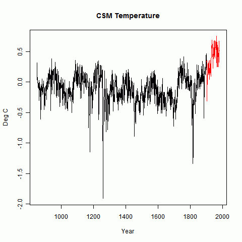
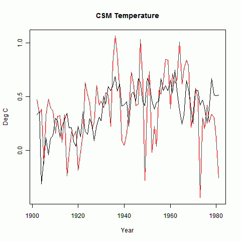
I created 59 proxies as described. The factors F, which are approx the S/N) were randomly generated in a range from 0.03 to 0.18. Once generated these factors were kept constant through the analysis. Unit white noise was added and the result normalized.


I'll show first the temperature, with calibration period in red. There's not much point in showing a bare proxy - it just looks like noise.





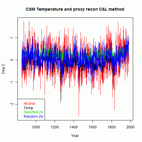
The next plot shows, in red, the CPS recon as described above. The green is an "unbiased" recon where T has the corresponding amount of white noise added.





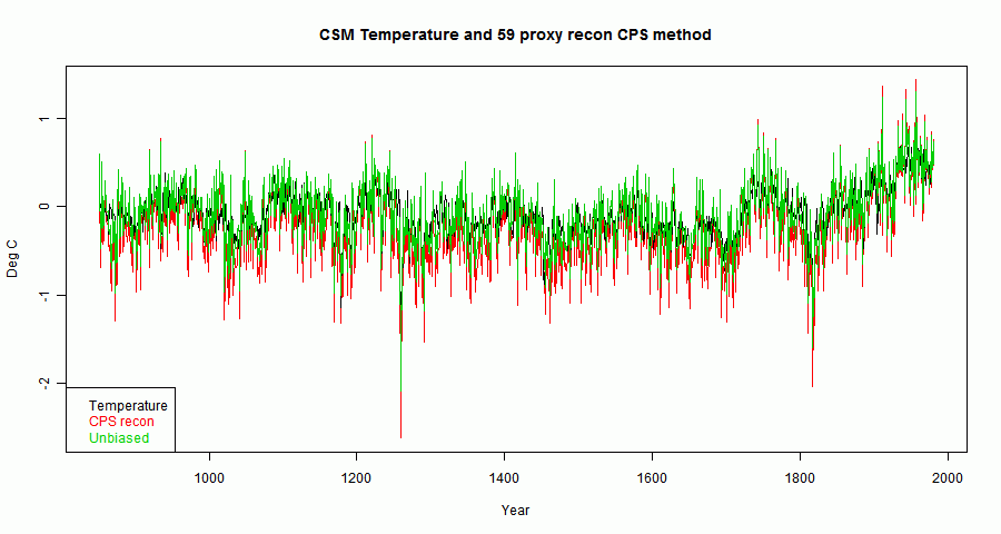
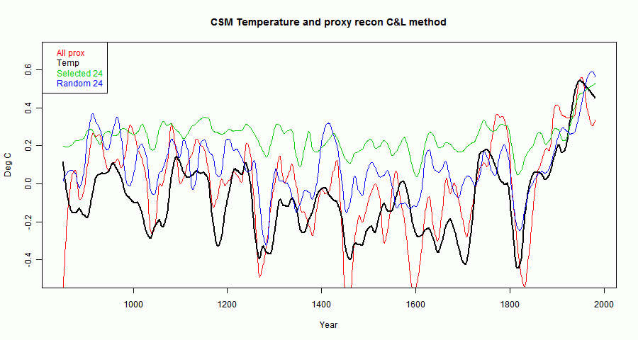
Noise is dominant, but the HS shape is there, reflecting the way the proxies were constructed. A smoothed curve will show any biases better (emphasising them greatly relative to the noise):

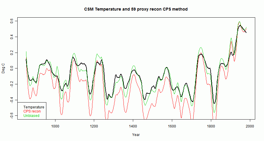
Update. I originally had colors wrong on the legend. To fix this, I did a new run. As I say below, the apparent "bias" can go either way - in the earlier plot it was above by a large margin; this time it's below. I've changed the relevant numbers.

There is a small apparent bias in the scale factor which multiplies the green curve to get the red. This is the \(1+e\cdot T\) denominator and can go either way. In this case, the se for this is about 0.14 about a mean of 1. In fact in this realization it was 0.83, which is on the low side.

There is an actual bias, because of the non-linear operation of inversion. However, in this case it is only about 0.02 - ie 2% difference.

Selection

So now what happens if a subset of proxies is chosen according to the correlation in the calibration period? The correlation, with above normalizing and notation, is:
$$\rho_i=P_i\cdot T = F_i+w_i\cdot T$$
The intent of selection is to choose for high S/N - ie F. But the selection cannot distinguish between ρ that is high for this reason or high because of the second factor - a chance alignment of noise with T in the calibration period. One of these will persist pre-cal, the other probably will not.

Note that this effect is dependent on the distribution of F values. If they are all equal - a common choice for toy examples - then the effect is maximised, because selection is purely on the random alignments of w and T. And if the S/N is low, again random will dominate. But if there is a subset with high S/N, then selection for these will work as intended, and create little bias.

So in the recon, the denominator \(1+e\cdot T\) no longer has expected value 1, and so is a source of genuine bias. Let's see how that works out, choosing the top 24 by calib ρ out of the 59:





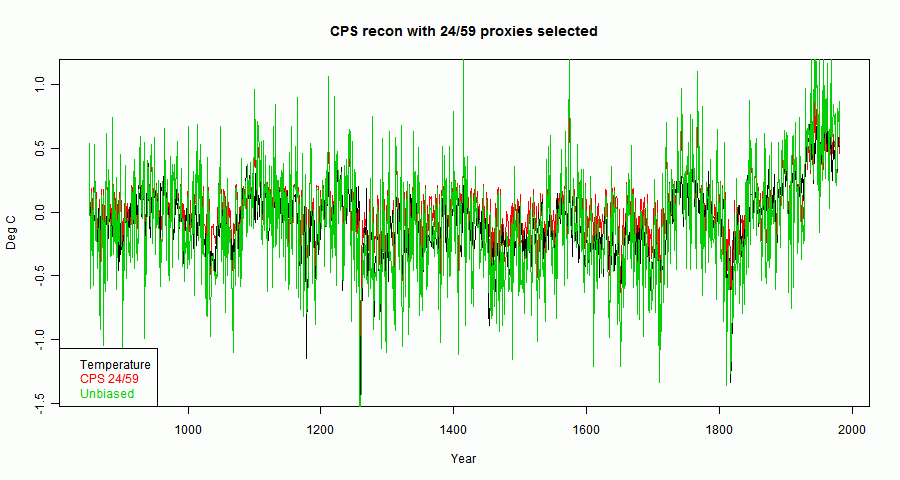
You can see that the red now lies abobe the black and green, clearer in a smoothed plot:





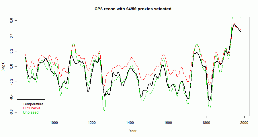
In fact, the denomninator \(1+e\cdot T=1.66\) which is the source of the bias.

Implication

Having identified the source of the bias, it would be nice to be able to correct for it. However, the denominator involves f which is the very thing we are after.

The main thing to say is that for CPS, the only case analyzed here, the effect is not so important, because selection by correlation after normalization is not usually done. A variant which may be of some importance is where a correlation-weighted sum of proxies is used.

Code is here

Paleo reconstructions and the "selection fallacy"

I've been arguing again, this time at CA and Lucia's. There's a series of threads of which I've linked the latest. The issue arose in connection with the SH proxy paper by Gergis et al, recently famously taken back for repairs (so I can't link to it). The method issues are described in an extant paper by Neukom and Gergis, 2011.

The issue is a claim that a common practice of making a last-stage proxy selection by observed correlation with temperature in the calibration period (when instrumental readings are available) constitutes a "selection fallacy". I made myself unpopular by asking just what that is - the response seemed to be that I'd been told and anyway any right-thinking person would know.

But there have been attempts to demonstrate it, with varying effects, and whatever the "fallacy" was, it seems to be shrinking. Lucia says now that she doesn't object in principle to selecting by correlation; only to certain methods of implementing. There was an interesting suggestion at CA from mt to use MSE rather than correlation for selection.

Roman's CA example, linked above, was held to show a selection bias. But it turned out that there is in his CPS method a bias from the limited number of proxies, and selection by correlation had no more evident effect than random selection. He then gave another example with white noise and more proxies with higher S/N which did seem to show some selection effect.

Anyway, I've been doing some tinkering with methods, which I'll describe.

Proxy reconstruction

For general information about proxy methods, I've been referring to the NRC CommitteeNRC North Report. I find this a useful source precisely because it is a panel effort, with a contribution and review from noted statisticians (who did not seem to notice a "selection fallacy"). The basic task is to get as many proxies as you can, form some sort of average and scale it to temperature. The scaling necessarily involves a correlation with some measure of instrumental temperature. Proxies are any observed property of which you have a long and dateable history, which you expect to be primarily influenced by temperature in a relation that could be expected to have endured.

An obvious problem with averaging the proxies is that they may be diverse properties, even with different units. One method, popular in times past, is CPS, which normalizes and averages. Normalizing means to scale with zero mean and unit variance.

A problem with this, not so often noted, is that the proxies are not stationary random variables, for which a notion of variance makes sense. They do, or should, echo temperature (which also gets normalized), and this has a strong secular trend, at least recently. Normalizing sounds normal, but it is weighting. Since it usually involves dividing by the sd taken over all available time, that weighting does involve peeking at the period of time for which you want results. In particular, it downweights proxies that show variation due to features like the MWP.

A less obvious problem is overfitting. There is a century or less of annual data available, and this may well be less than the number of proxies you want to scale. CPS, which reduces to one series, was favored because of that. Selecting proxies by correlation also counters overfitting.

In my view, the first method of aggregating considered should be to scale the individual proxies by imputed temperature. You can do this by some kind of regression against temperature in the overlap period. I believe this is what Gergis et al did, and it requires that you find a statistically significant relation to proceed. IOW, selection by correlation not only reduces overfitting, but is required.

Carrick noted a very recent paper by Christiansen and Ljungqvist 2012 which follows this method. In this post I experiment with that method.

Regression issues

Since you eventually want to determine T from P (proxy value), it might seem natural to regress T on P. This is CCE (Classical Calibration Estimator). But people (eg MBH 1998) use inverse calibration (ICE) of P on T, and C&L recommend this as being more physical (P is (maybe) determined by T).

It makes a difference. Since P and T are both subject to what is normally modelled as error, when you choose one as the regressor, the combined error tends to be attributed to the regressand. So CCE tends to inflate the variance of T, and ICE tends to deflate it. But the method normally invoked here is EIV - Errors in Variables.

EIV can be pretty complex, but there is a long-standing one-regressor version called Deming regression (not invented by Deming). The key problem is that you want to find a line that minimises least square distance from a sctter of points, rather than distance ot one of the axes. The problem is, that line depends on the axis scaling. In Deming regression, you scale according to the estimated variance of each of the variables.

Deming formulae

We need to regress over a calibration period. I'll use subscript cal to denote variables restricted to that period. For the i'th proxy, let
$$xm=mean (T_{cal});\ \ x=T_{cal}-xm$$
and
$$ym=mean (P_{cal});\ \ y=P_{cal}-ym$$
We need the dot products
$$sxx=x\cdot x,\ \ sxy=x\cdot y,\ \ syy=y\cdot y$$
Finally, we need an estimate of the variance ratio. I could use $$d=syy/sxx$$. That actually greatly simplifies the Deming formula below - the slope reduces to \(\sqrt(d)\). However, because x and y aren't anything like stationary, they should at least be detrended to estimate d. I prefer to subtract a smoothed loess approximant (f=0.4); it generates a ratio of high frequency noise, but at least it seems more like noise.

Then the Deming formula for slope is
$$\hat{\beta}= w+\sqrt{w^2+d},\ \ \ w=(syy-d*sxx)/sxy/2$$
and the best fitted T is
$$T=xm+(P-ym)/\hat{\beta}$$
Note that I've dropped the cal suffix; this is the best fit in the calibration, with the formula extended.

Noise

The results without screening, in the example below, seem very noisy. The reason is that when correlation is low, the slope is poorly determined. My next exercise will probably be to weight according to regression uncertainty. But for the moment, I'll stick with screening as a method for reducing noise.

Example

I'm using Roman's example data. This consists of CSM modelled temperature with 59 proxies (850-1980) taken from a paper by Schmidt et al, with realistic noise added to the modelled temperature. A 26 Mb zipped datafile is here.

The selected group were those with correlation exceeding 0.12. There were 24. I also included a non-selected group of 24 (proxies 10 to 33).

Fig 1 shows the temperature in the screening period, which like Roman I took to be 1901 to 1980.



Fig 2 shows the full reconstruction. It mainly shows that the selected group came out somewhat higher, and the full proxy set is very noisy.



Fig 3 shows the reconstruction, but using Roman's smoother. It makes things clearer. The unscreened versions seem relatively unbiased but noisy. The screened version looks rather like Roman's CPS version, and has slightly smaller MSE (0.17).



I'll post the code tomorrow. This post is technically somewhat interim - I want to explore the effect of weighting according to regression uncertainty.

Update - code is here

May GISS Temp up 0.1°C - ice news

TempLS showed changed very little from April to May. GISS showed a rise, from 0.55 °C to 0.65 °C. GISS has been rising steadily, while other indices that showed bigger rises in March/April have paused. Time series graphs are shown here

In other news, you should check that link for the Arctic ice changes over the last week. Ice was holding up well, but has dived to a record low for this time.



As usual, I compared the previously posted TempLS distribution to the GISS plot.
Here is GISS:


And here is the previous TempLS spherical harmonics plot:

Previous Months

April
March
February
January
December
November
October
September
August

More data and plots

TempLS: May temperature same as April

The TempLS analysis, based on GHCNV3 land temperatures and the ERSST sea temps, showed a monthly average of 0.53°C for May, unchanged from April (April rose by a few thousandths with late data). UAH also was virtually unchanged. It was still very warm in much of NH, including the Eastern USA. There are more details at the latest temperature data page.

Below is the graph (lat/lon) of temperature distribution for May.






This is done with the GISS colors and temperature intervals, and as usual I'll post a comparison when GISS comes out.
And here, from the data page, is the plot of the major indices for the last four months:

Arctic Ice Volume Anomalies

I made a small and somewhat inaccurate contribution to another WUWT thread, this time on Arctic Ice volume, and a figure quoted by the Guardian which I found surprising. My error is explained here; Stoat's account of the matter is here.

Anyway, it made me realise that I should pay more attention to ice volume. Although I criticise the Guardian's 75% reduction since 1979 as a mild exaggeration, the mean reduction of 66% is still an impressive figure. So I downloaded the PIOMAS data, and put it through the anomaly visualisation program of my previous post.



Again there are two anomalies calculated - without and with trend adjustment. The trend this time is much larger, so you need to watch the units.

Here's the analogue of the familiar Jaxa plot with the fitted periodic annual curve. It isn't an anomaly, and there is no detrending. You can see the steady downtrend, and I've shown the y-axis based at zero, so you can see it isn't so far off.



2012 is marked in black.

Here is the anomaly plot with trend, shown over the years from 1979:



You can't now see where ice-free is, but the persistent trend is evident, with some recent acceleration.

Now here is the same data plotted over a one year interval. Again 2012 is black. The ice volume is pretty much as last year, which is bucking the trend a bit.



Plotting the anomaly after allowing for trend gives a similar picture, but note the lower y-range. Over the last two years, mid-year has been a marked minimum of the anomaly, but this year (as at end April) it has not yet started that dive.

Sea Ice anomalies

Since Jaxa resumed posting daily results of Arctic Sea Ice extent, I've been processing the data and posting plots here. I'm thinking of doing an interactive plotter for the various ice measures, similar to the climate plotter.You could choose which years to show.

So I started looking at means and anomalies, and thinking about trend calculations. The general method for anomalies seems to be to take a day-by-day average over some years and calculate discrepancies from that. The number of years is not huge, and there is a spike of variability near the maximum melt, so the daily mean is not free of the fluctuations from which an anomaly is sought. So I tried a multiple regression using trig functions and a secular trend.

An anomaly plot is useful for plotting in that it removes the seasonal oscillation, making the key information more visible. With the trig functions I can use a sidereal year, which gets rid of a minor but awkward leap year issue. I found four harmonics was sufficient as the magnitudes taper quite fast; using five made negligible difference.

I looked at the Jaxa data, and also the Arctic and Antarctic sea extent data from UIUC (Cryosphere Today).



There are two anomalies calculated - without and with trend adjustment. All curves have been very slightly smoothed, with a 5-point binomial filter.

JAXA IJIS

Here's the familiar Jaxa plot with the fitted periodic annual curve.

2012 is marked in black.

Here is the anomaly plot with trend, shown over the years from 2002:

The downtrend is about 65000 sq/m/year. Last years minimum was about 4500000sq km; at that rate of attrition it will be nearly 70 years before it disappears. However, there's no reason to expect that trend to apply over the period, and indeed the minima seem more variable than the general trend.

Now here is the same data plotted over a one year interval. Again 2012 is black. It shows that the anomaly so far this year is mid-range for the decade.


However, plotting the anomaly after allowing for trend shows that so far, 2012 is rather higher than expected.

UIUC Cryosphere Today Arctic

UIUC published data over a much longer period. They do their own anomaly calculations, which are in the data set and published on their website. But these are from the trig function regression. Here is the anomaly plot over years:

The trend is somewhat less than Jaxa, since the period is three times longer. Now the same plot superimposed.

There are now a lot of curves, so I've shown the last ten years with greater thickness.

Finally the trend-removed anomaly plot. Again 2012 is currently fairly high relative to recent years.

UIUC Cryosphere Today Antarctic

Finally, for completeness, the Antarctic data. They are of course six months out of phase, and the trend is up rather than down, though the magnitude is less than Arctic. Here are the anomalies:


The same over years:

and with trend removed:

I've been paged

Again
at WUWT

I responded there at about 7.30pm 29 May here (2.30 am PDST). My posts there now just disappear - I think into the spam bucket. We'll see if it appears.