New text and file repository

Over on the right, under Resources, there is a link to a "Document Store". That's where I keep various bits of code and other texts. The TempLS material is there, for example. I had been keeping it on a location on drop.IO.

Steve Mosher warned me that drop.IO has been taken over by Facebook, and will be closing. I looked around, and discovered that there is a much better alternative. Google Sites allows users, free, to set up a site with 100 Mb of space, to which you can upload files, images, etc. It also offers a range of templates replete with gadgets.

So I have set one up. It's a bit of a work in progress. The templates are impressive, but none quite matched. I chose a project template, which has lots of facilities, but some not really appropriate management talk. I've tried to keep that to a minimum.

So if you go to the new Document store you'll see a home page, with some intro stuff (not much yet), and a pointer to a page of "Project Documents". This is the new repository. The Google facility allows me much more freedom in writing descriptive text (so I'll have to do it :().

I'll also use it to host images - I've set up a "Picture Gallery". There's no real reason to look at that, as it's just for images to link in to posts, but you can if you want. I had been using TinyPic, but I don't need to do that any more.

I'll also transfer to it ongoing items like the category index of posts, and the temperature tracking page. I'll also make an updated TempLS page and keep it there.

The links within past posts still point to drop.IO, and I probably won't fix many of them. But you can always use the link under resources.

One merit of the new scheme is that I can link to individual files.

Woody Guthrie Award - thanks, Science of Doom

A note to thank Science of Doom. I am very honoured that he has chosen this blog  as his successor,  with the privilege of passing on the Woody Guthrie Award. I was especially pleased because SoD's style of dispassionate informative blogging is what I have aspired to here. So thanks, Science of Doom. And thanks to readers, who keep this blog going.

I did a bit of googling to find the history of the award, which I have been aware of since it first came to Skeptical Science. I've been able to track it back a few generations, as far back as Ærchie's Archive, who passed it on to Honji's Harangues. From there it went to honestpoet at
Enough is Enough, and she nominated Greenfyre's.
 
This was an interesting change, from a succession of rather philosophical blogs to one with a science/climate focus.

Greenfyre's passed it to Dan's Wild Wild Science Journal, who then passed it to
Skeptical Science. They awarded it to Science of Doom and, well, here we are.

Unfortunately, I can't find a reference to the event on Ærchie's Archive, so I can't go back further. But the search took me to a lot of interesting blogs, of which Archie's is one. It's discursive, but with a focus on Perth landscapes and history. I like Perth a lot - I've lived there - and I think Archie gets it well. Currently active and recommended.

The award used to come with a little graphic;



which may have been more relevant in its earlier life cycle.

Anyway, it's now my job to pass it on. No need to rush there but thoughts would be welcome. Given its history, it seems ideas need not be restricted to the climate science community. I would have given a lot of thought to this excellent blog, but sadly, the owner retired a few months ago. I miss it.

Condensation - the Eulerian View

In the previous post I analysed the effect of expansion in a cylinder on condensation. As the pressure reduces, of course, the volume increases. The key question was whether it increases more or less than if the air had been unsaturated.

This is supposed to help with what might happen in atmospheric uplift, as in a hurricane. The pressure reduces and the gas expands in the same way. If you focus on the moving air, in fluid mechanics that is the Lagrangian view.

It's better for intuition - the boundaries of the volume travel with the fluid, and by assumption in the atmosphere, heat and other species like water vapor travel with it too, and remain in the boundaries.. That is because diffusion over the large distances is relatively small, although thermal radiation could be an issue.

But there are problems when you want to think about the processes in relation to other things that are not moving with that fluid. Fixed boundaries are one issue - not so common in the atmosphere. But in the ongoing argument about Anastassia Makarieva's contraction theories (TaV1, JC and TaV2, Lucia1, Lucia2),  AM prefers the Eulerian frame, a fixed volume in space.

The good thing there is that you can assume steady conditions. At every point the velocity, temperature etc will remain steady, even though as you follow it in the flow, it changes. The bad thing is that the boundaries are no longer material boundaries, and you have to account for whatever is crossing it. Not so intuitive.

Scientists tend to talk Lagrangian to students, but Eulerian to their computers.

Here I'll take the Eulerian view of expansion and condensation.

A 1D (vertical) problem

In accounting for boundaries, it helps to have only two (upper and lower). I'll look at a 1 m thick slice, assuming zero horizontal gradients. The notation is generally as in the previous post. We'll say z goes from 0 to 1, and I'll suffix accordingly (but if suffix is missing, assume zero). So T,V,P, ρ are assumed known at z=0. The incoming air is saturated.

I'll also assume, as is conventional, hydrostatic pressure. So P₁ =P₀ -ρ g

Then each incoming packet of air changes according to the cylinder analysis, with this pressure increment:

T₁ =T₀ -ρ g dT/dP

where dT/dP = (T/P) DT/DP = (T/P) (1+c+c/b)/(3.5+b+b*c), b=L/(R*T), c = b*n_w/n
In the previous post, n, n_w were moles in a volume V. Here I'll take V=1, so they are molar densities.

n_w1 =n_w0 -ρ g dn_w/dP

where dn_w/dP = (n_w/P) Dn_w/DP = (n_w/P) (1+c+c/b)/(3.5+b+b*c)

Density is calculated from dV. The mass change in the unit volume element M_w*dn_w,  ( M_w = molar mass of water) so the density change is

d ρ /dP = M_w*dn_w /dP + ρ/P DV/DP

= (M_w*n_w /P *(b-3.5)+ ρ/P (2.5+b*c+2.5*c/b-c))/(3.5+c+b*c)

Velocity and precipitation reconciliation

The molar mass flux of dry air through z0 is    v₀*N_d
The number of moles is conserved; in the notation of the previous post, N_d varies inversely as V, ie DN_d/DP=-DV/DP.
So with v=1 m/s,
dv/dP=(v/P)Dv/DP = (v/P)DV/DP=(v/P)a4/a3
Velocity v increases with z.

The precipitation rate r moles/m³/s is

r=v dn_w/dz= vρ g (n_w/P) (1+c+c/b)/(3.5+b+b*c)

Results

Again the meaningful test is to compare saturated air with unsaturated air under the same conditions. With z in km:

	dT/dz	dnw/dz	dρ/dz	dv/dz
Dry	-9.75	0	-0.0937	0.0818
Sat	-4.151	-0.147	-0.1137	0.0969

The results are much as expected. dT/dz is the lapse rate. dn_w/dz is numerically (withv=1) the precipitation rate in moles/km/m²/sec . 0.147 is equivalent to 9.5 mm/hr from a 1 km column - but remember the 1m/s velocity is arbitrary. The density reduces with height, but more rapidly for the saturated flow. And the velocity also increases more rapidly.

Interpretation

It is a steady flow. But also expanding. The upward velocity would have increased just because of the hydrostatic density gradient, but it increases more because of the condensation. This is due to the release of latent heat, which dominates the contraction due to mass loss.

The same expansion is seen in the density gradient (reducing faster). and the warming is seen in the well-known reduction of lapse rate with condensation.

Further note

 I mentioned in the previous post that the formula for DT/DP could be found, with slight modification, in the Phys Met notes of Dr Caballero. I realised then that it is just the formula for the saturated adiabatic lapse rate, which has a much longer history.

As explained in that earlier post, my form isn't quite the same. There is a discrepancy due to the mole concentration I made in the Ideal Gas Law. I've kept with it, because it does seem to be the irght thing to do.

R Code

 T=298.15
V=v=1
P=98131
R=8.314
N=P*V/(R*T)
Nw=0.03128*N 
Cv=20.85
Mw=0.018
Ma=0.02896
L=2304900*Mw
g=9.8
rho = N*Ma
 
b=L/R/T
c=b*Nw/N
a1=1+c+c/b
a2=b-3.5
a3=b*a1-a2
a4= -(2.5*a1+c*a2)
 
dp=c(0,0,0,0)
dp[1]=dTdP=(T/P)*(a1/a3)
dp[2]=dNwdP=(Nw/P)*(a2/a3)
dp[3]=drhodP  = (Mw*(Nw/P)*a2 - (rho/P)*a4)/a3
dp[4]=(v/P)*a4/a3
dz=-dp*rho*g*1000
# print(dp); print(c(a1,a2,a3,a4))
print(dz)

Condensation and expansion

There has been much blog discussion of whether condensation of water in the atmosphere is accompanied by a volume expansion or contraction. Standard theory says expansion, but Anastassia Makarieva has been promoting a theory that winds are driven by contraction caused by condensation. There is discussion here and here. The paper (M10) is available and open for online discussion here.

M10 has a whole section devoted to demonstrating that a fixed adiabatic volume cannot undergo condensation. As I'll show, this is an unsurprising result. But the section arises from reviews of an earlier paper suggesting hurricanes were driven by condensation-induced contraction. Reviewers objected that latent heat release would outweigh the tendency to contract to to loss of water vapor volume. So there was no contraction to provide energy.

On the Air Vent threads, various experiments to study condensation/contraction were proposed involving air in bags and bottles, etc. I have been trying to explain how they lack the adiabatic expansion that causes cloud condensation. Bodies of air rise, and as they do so they expand, doing work and cooling. If they are saturated with water vapor, some of this condenses. Because the cooling is adiabatic, the latent heat is retained and slows down the cooling and condensation process. The result is that the air parcel becomes warmer than its surroundings (though cooler than it was originally) and so expands relative to nearby air.

Below the jump, I'll describe a stationary volume-change process with condensation, and calculate the expansion effect.



Consider a volume of saturated air held adiabatically in a chamber with a piston which can force an expansion. For definiteness, let's say that  V=25 m³ at T=300°K, containing n=1000 moles of air+water at P=100 kPa. Latent heat (of vap) L=45 kJ/mol. There are n_w =36 moles of water vapor present.

As the piston moves, there are three governing equations:
Conservation of energy

1)      n c_v dT + L dn_w + P dV = 0

Ideal Gas Law:

2)     P dV + V dP = n R dT + dn_w RT

Clausius-Clapeyron Equation

3)     RT² dn_w = L n_w dT (see update)

[Update - a small error here. I've identified  dn_w/n_w with dp_w/p_w  But in fact
p_{w =p(}n_w/n) .and p is not constant. So it should be
3)    RT² (dn_w/n_w + dp/p)= L dT
It makes a small difference - full update to come (7.47 am 9 Nov)
It's here (140 pm) - I've marked new in brown, and obsolete in grey]

I prefer to put these in non-dimensional form, using a notation Dy =1/y dy (y=T,P etc). That means that Dy is a proportional change in y. So:

Divide (1) by PV or nRT

4)     c_v/R DT + (L*n_w)/(R*T*n) Dn_w + DV = 0

Divide (2) by PV or nRT
5)      - DT - n_w/n Dn_w + DP + DV = 0


Divide (3) by R*T²*n_w

6)      - L/(R*T) DT + Dn_w + DP = 0

Solving

There are three equations in the four variables (DT, Dn_w, DP, DV). However, one of these, DP or DV, is specified (the amount the piston is moved).

If you set DV=0, then there is just one solution DT= Dn_w=DP=0. In other words, no condensation - nothing can happen. That's what Sec 2 of M10 was about.

Fixing DP is most natural for atmospheric comparison, since P is a measure of altitude. Dividing the equations by DP gives the derivatives ( DT/DP, Dn_w/DP, DV/DP). Remember these are proportional derivatives. If you change P by p%, then you change V by (DV/DP)*p %.

I did a first solution with n_w=0. This is in effect the dry air case. The R code is below.

With the diatomic c_v/R = 5/2, it gave, as expected,
  DT/DP=2/7=0.2857,    DV/DP=5/7= -0.714
That means that if P decreases by 1%, then the volume V increases by 0.71% and T decreases by 0.28%

Then I did the solution for the above case at 300 °K, 100 kPa. The answers were:

DT/DP=0.063,    Dn_w/DP=1.14,      DV/DP=-0.896

DT/DP=0.106,    Dn_w/DP=0.916,      DV/DP=-0.861

Added: Plot of % variation (dry and wet) of temp, volume and wv with varying P. Note that with expansion, P diminishes.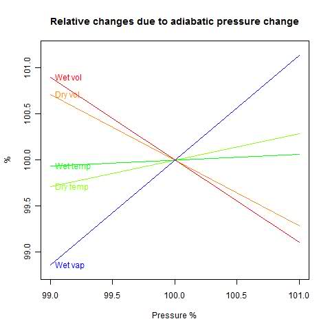

First observation - wet DT/DP is much smaller. Condensation is stabilizing the temperature, as you'd expect. And a 1% drop in P causes 0.916 1.14% of water vapor to precipitate.

But the answer I was looking for is the third. A 1% drop in P increases the volume by 0.861 0.896% - more than it does for dry air (0.714%). The condensation causes the volume to expand relative to non-condensing air.

Interpretation

This study was just of air in a confined space. But it can be applied to saturated air rising in parcels in the atmosphere. The dry lapse rate is the temperature gradient which is neutral for air moving without condensation (more here). So the moist air is cooling more slowly than the lapse rate as it rises, and is expanding relative to air on its level.

Update - more algebra

Equations 4-6 can be rewritten in even fewer non-dimensional parameters. I'll take the ratio c_v/R = 5/2.

Then with b=L/(R*T), and c=(L*n_w)/(n*R*T)

7)      2.5 DT + c Dn_w + DV = 0

8)      - DT - (c/b) Dn_w + DP + DV= 0

9)      -b DT + Dn_w + DP = 0

Eqns 7-9 are linear homogeneous equations in the four variables: (DT, Dn_w, DP, DV) The answer can be expressed in terms of a vector a=( a₁,a₂,a₃,a₄ ) and an arbitrary parameter h:

DT=a₁h,  Dn_w=a₂h,  DP=a₃h,  DV=a₄h. 

Finding a is a matter of linear algebra (school algebra or determinants). I'll just state the result and verify:

a₁ = 1 + c + c/b,  a₂ = b - 3.5,  a₃ = 3.5+c+b*c,  a₄ = -(2.5+b*c+2.5*c/b-c)

Substitute in (7) with h=1 (h will cancel):

2.5*a₁ + c * a₂  + a₄  =  2.5+2.5*c+2.5*c/b + c * b-3.5*c - 2.5 - b*c+-2.5*c/b+c  =  0

And (8): -a₁ -(c/b)* a₂ + a₃ + a₄  =  1- c-c/b  - c+3.5*c/b + 3.5 + c + b*c - 2.5 - b*c-2.5*c/b+c  =  0

And (9): -b*a₁+ a₂  =  -b-c-b*c + b- 3.5 + 3.5+c+b*c = 0

You can use this result to get any desired derivative, eg DV/DP = a₄/a₃. 

Remember again that D is proportional, so dV/dP = (V/P) a₄/a₃.

Update. I see that Eq 3.74 of Rodrigo Caballero's PhysMet lecture notes gives a version of DT/DP which is equivalent to (1+c)/(3.5+bc). He says this is an approximation (3.72). I think that is equivalent to omitting the last term in my Eq 2, which would indeed give this expression. However, I believe the inclusion of that term is more accurate.
 

Appendix - R code

V=25
T=300
N=1000
Nw=36   #0
P=100000
R=8.3
Cv=R*2.5
L=45000

LRT=L/R/T
m=matrix(c(Cv/R,-1,-LRT,  LRT*Nw/N, -Nw/N,1, 1,1,0, 0,1,1),3,4);

M=m[,c(1,2,4)]; rh= -m[,3];
ddV=solve(M,rh);    # D/DV volume derivatives


M=m[,c(1,2,3)]; rh= -m[,4];
ddP=solve(M,rh);    # D/DP pressure derivatives

print(ddV);  print(ddP);

A ramble on GCMs Navier-Stokes equations.

This post is an outgrowth of a discussion at the Air Vent on GCM's and condensation. It's a kind of response to comment claims that GCN's don't allow for inversion, or volume change during condensation etc. I found myself saying often that it all comes out in the solution of the Navier-Stokes equations - you don't have to do something special.

It's often said that the N-S equations are at the heart of GCM's, but if you look at a set of equations actually solved, as in this set from CAM3, it isn't obvious. And it's made less obvious by the funny coordinates they use.

But it's true, and here I'll try to set out the reasons.

The Navier Stokes equations

These go back to Navier in 1822, although his physics was eccentric, based on a stretched version of recent atomic theory. GG Stokes in about 1845 gave a definitive derivation and solved most of the special cases that could be done theoretically. In the mean time, Poisson and Saint-Venant also made big contributions. In fact, what I'll be talking about mainly goes back to Euler.

I'll write out a version for slightly compressible fluids. An abstract form is:

ρDv/Dt = -∇.τ	Momentum equation
Dρ/Dt = -∇.(ρv) Mass	conservation or continuity
ρ-ρ0=(P-P0)c-2	Constitutive Relation

Update - I've added a P0 to that last equation (I'm used to thinking of ambient pressure as 0, but of course in the atmosphere that won't do).  At Lucia's suggestion I've used the more orthodox term constitutive relation (not eqn of state). I'll also mention that ρ is density, v velocity, P pressure and t time.
D/Dt represents a total or advective derivative - in a frame moving with the fluid. ∇ is a vector derivative operator (∂/∂x,∂/∂y,∂/∂z), and τ is a stress tensor. Don't worry about what that means if it's unfamiliar - it's about to disappear.

I've chosen this "abstract" style to show the structure. The momentum equation is just Newton's second Law -   ma = F . Continuity just says that if mass is moved by advection (being carried with the flow), the density will change. And this constitutive relation just says that to change the density from a standard (local hydrostatic) value, you have to apply a pressure P, and c is the speed of sound. You could have other constitutive relations for different materials.

The stress tensor could be quite complex, but for now, let's just say there's a pressure P, gravity g, and a viscous stress (coef μ). Atmospheric flows are always turbulent, and turbulence models can work by modifying the viscosity. But I mainly want to talk about the pressure-velocity interaction, so I'll just keep a viscous term as an example of the other things that could come in.

OK, so now we have:

ρDv/Dt = -∇P + ρg + ∇.(μ∇v)	Momentum equation
DP/Dt = -ρc2∇.(v)	Mass conservation or continuity

Time Scales and numerical solution

Suppose you wanted to solve these numerically. You'll have the space divided up into regions, with the field variables (P, v etc) represented on nodes - maybe the corner points. You'll have linear expressions for the space derivatives in terms of nodal values.

So a naive approach is to say - suppose you calculate the right hand sides at a point in time. just calculate the rates of change of v and P, and assume that holds for a timestep. Update and proceed. That's called an explicit method (forward Euler).

But it won't work, except for very small time steps. The reason is that, while you've got starting information within your little regions, what's going on in one region can affect others during that step. You're limited by the fastest process that can propagate physical effects. And that is the speed of sound, which is the way pressure is propagated.

The reason is that buried in the N-S equations is the acoustic wave equation:

ρdv/dt = ∇P

dP/dt = -ρc2∇.v+...

or

c-2d2 P/dt2 = ∇2P+R1

or

c-2d2v/dt2 = c2∇2v +R2

I've replaced D by d, because only fast processes are retained, and the difference between D and d is an advective term, which is also slow relative to sound speed. R1 and R2 denote the slow terms.

By small time steps, I mean small enough so that a sound wave will only move part way across one of the small regions. In GCM's, the vertical divisions can be just a few hundred metres. That's a second or so of sound time. That would be ridiculously short for GCM modelling, where steps of about half an hour are common. Incidentally, these are constrained by the speed of other "weather-like" processes.

Coupling and semi-implicit solution

The problem is that with the explicit method, we have to resolve the acoustic oscillations, which are not of interest.

Looking at the pressure wave equation, we can say that, since c is large, only acoustic solutions will have a significant left side. For the solutions we actually want, that can be dropped. Then we get

∇²P  = - R1

wher again R1 is a collection of slow terms. This is what is called the Pressure Poisson equation. Once solved, the pressure can be used to get the velocity by going back to the momentum equation.

The essential thing here is taking the pressure and velocity equations together - coupling. Everything else can be held constant during the time step (though you can also do better with staggered time steps etc - there's lots of extra art not relevant here).

So now the time step can be extended until the next fastest process will mean that the computational cell cannot be regarded as (sufficiently) isolated during the timestep. Since that process is generally, unlike sound, one of the processes you do want to resolve, that's basically it.

Summary

So that's why the Navier-Stokes equations are the core. They can be seen as an engine that matches pressure and velocity, using sound implicitly, but not requiring sound-limited timesteps. Once you have that sorted out in a time-step, all the other physical processes can be updated in good time.

Heretical afterthought - for practitioners

Actually, implicit solution is not as rosy as it is often painted. You can take long time-steps, but you have to solve a big matrix of equations to do it, instead of just calculating new values at each node. You take advantage of the fact that each node only affects a few neighbors, which gives a sparse matrix. So for big systems you use an iterative solver.

The gloomy fact is that the iterative solver, in effect, is an accelerated version of the original explicit solution. And using something like conjugate gradients, the acceleration is significant, but not super. Preconditioning helps, as does a process called multigrid. But the fact remains that, as you extend the timestep, the matrix becomes more ill-conditioned (an analyst's curse word), and you end up with a number of iterations rather related to the number of explicit steps you would have had to perform.

I might say more about preconditioning in a future post.

Wahl & Ammann proxy calculations

I had been quietly plodding through Wahl and Ammann 2007. This is the paper that re-did the MBH98/99 proxy calculations using conventionally centred principal components analysis and a modified number of PC's. It's relevant to recent discussions of the Wegman report.

Some original code and data used in the paper is available at Nychka's site at NCAR. So I downloaded it. It's elegant in R. Just 11 lines of actual calculation to get from the proxy data to a set of proxy eigenvectors, with decentered scaling. And then, of course, R does the regular PCA for comparison in one line.

Then Ron Broberg put up a very helpful post drawing attention to a discussion by Dr Richard Smith of a recent paper by Li, Nychka and Ammann. As Ron says, it's well worth reading (as is Ron's post). I've only just started.

The R code

To get me going, I re-commented Ammann's code, to help my understanding. I'll show it, with the Figures, below the jump.

So the next stage is for me to recheck the things that are commonly said about the various proxies, and how they are reweighted. Later it might be possible to adapt the code for the Mann08 (Tiljander etc) analysis.



Here's Ammann's code for the decentred PCA. My comments have a double ##:
# read in data

## scan a big file of proxy data - 70 proxies, 581 years from 1400:1980
## North America
T<-scan("2004GL021750-NOAMER.1400.txt",skip=1)
T<-matrix(T,nrow=581,ncol=72,byrow=TRUE)
tree<-T[1:581,3:72]
## tree is the matrix of proxy data over 1:581 years (1400:1980) - 70 proxies

tt<- c(1400:1980)


# MBH- uncentered PCs  GRL Data, Caspar Ammann's code
# =======
## This part rescales tree according to the mean and sd to get xstd
m.tree<-apply(tree[503:581,],2,mean)
s.tree<-apply(tree[503:581,],2,sd)
xstd<-scale(tree,center=m.tree,scale=s.tree)
## regress 1902:1980 columns of xstd against years in calibration period
fm<-lm(xstd[503:581,]~c(1:nrow(xstd[503:581,]))) #fit linear model to calibrati$
## fm($residuals) is the set (79x70) of residuals
## sdprox(1:70) is the sd for each proxy over the 79 years
sdprox<-sd(fm$residuals)                         #get residuals
## so now the xstd are rescaled relative to the calib period.
## This creates the famous MBH98 decentering (note center=F)
mxstd<-scale(xstd,center=FALSE,scale=sdprox)     #standardize by residual stddev
## Now do the svd decomposition on mxstd  = u * d * v
w<-svd(mxstd)                                    #SVD
## w$u is the 581x70 matrix of ordered eigenvectors
## w$d are the eivals =  164.3 83.1 58.9 50 45.6 ...
PCs<-w$u[,1:5]                                   #Retain only first 5 PCs for c$
## At this stage, "retain" is just the number of PC's that we calculate
m.pc<-apply(PCs[503:581,],2,mean)
s.pc<-apply(PCs[503:581,],2,sd)
PCs<-scale(PCs,center=m.pc,scale=s.pc)
## Now each PC is rescaled to mean=0, sd=1, again on 1902:1980

## Now just plot - fig1() and fig2() are plot routines which also call princomp().
source("fig1.R") # only need to source these fucntion once if they
source("fig2.R") # are saved in your work space.

## I changed the output from pdf to jpg for html posting
jpeg("fig1.jpg", width=900, height=800)
fig1()
dev.off()

jpeg("fig2.jpg", width=900, height=600)
fig2()
dev.off()


Here's the routine for fig1(). Note the one-line calcs for the regular PCA:

`fig1` <-
function(){

par( mfrow=c(3,1), oma=c(6,0,0,0))
par( mar=c(0,5,2,2))

## This does the whole PCA by the covariance method (cor=F is the default)
## It returns the "scores" - ie the first 5 (here) principal components
PCs.3<- princomp(tree)$scores[,1:5]

## This does the PCA by the correlation method
PCs.2<- princomp( tree, cor=TRUE)$scores[,1:5]

## tt is 1400:1980. PCs[,1] is first PC. The scale() seems redundant
## but isn't, because it was previously scaled to the calib period.
plot( tt,  scale(PCs[,1]), type="l", lty=1, xaxt="n", ylab="Scaled PC1")
abline(h=0,col="blue")
title("MBH centering and scaling in instrumental period",adj=0)

plot( tt,  -1*scale(PCs.3[,1]), type="l", lty=1,xaxt="n", ylab="Scaled PC1" )
abline(h=0,col="blue")
title("First PC using covariance",adj=0)


plot( tt,  scale(PCs.2[,1]),

type="l", lty=1, xaxt="n", ylab="Scaled PC1")
abline( h=0, col="blue")
title("First PC using correlations",adj=0)


par( oma=c(0,0,0,0), mar=c(5,5,2,2))
axis( 1)
mtext( side=1, line=3, text="Years")

}


Here's the resulting plot:

Here's the routine for fig2():

`fig2` <-
function(){

par( mfrow=c(2,1), oma=c(5,0,0,0))
par( mar=c(0,5,3,2))

## as for fig1()
PCs.3<- princomp(tree)$scores[,1:5]

PCs.2<- princomp( tree, cor=TRUE)$scores[,1:5]

## Plot the decentred MBH PC1
plot( tt,  scale(PCs[,1]),
type="l", lty=1, xaxt="n", ylab="Scaled PC1")
abline( h=0, col="blue")
title("First five covariance PCs projected (green)
  onto MBH centered and scaled PC (black)",adj=0)

## Regress the covariance PCs against decentred
lm( scale(PCs[,1]) ~ PCs.3[,1:5] ) -> out
## Plot the resulting fitted curve
lines( tt, predict(out), col="green", lwd=2)
lines( tt, scale(PCs[,1])) ## ?? this just seems to replot the MBH PC1

## Same, but done for the correlation method
plot( tt,  scale(PCs[,1]),
type="l", lty=1, xaxt="n", ylab="Scaled PC1")
abline( h=0, col="blue")
title("First five correlation PCs projected (green)
  onto MBH centered and scaled PC (black)",adj=0)

lm( scale(PCs[,1]) ~ PCs.2[,1:5] ) -> out
lines( tt, predict(out), col="green", lwd=2)
lines( tt, scale(PCs[,1]))

par( oma=c(0,0,0,0), mar=c(5,5,2,2))
axis( 1)
mtext(side=1, line=3, text="Years")

}


Here's the plot:

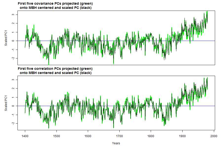I'll comment more on the results in the next post, and also look in more detail at the various PC's.

Can downwelling infrared warm the ocean?

Science of Doom has raised this question, which does crop up more frequently than it ought. Doug Hoyt, who should know better, has given it impetus.

It goes like this. Water is opaque to thermal IR, and not a good conductor. IR penetrates only a few microns. Therefore heat from incident IR from above must ...

be all converted to latent heat

or, be reflected, or ...

Land is also opaque to IR, but the idea that IR can't warm it doesn't seem to have the same attraction

Some thoughts below the jump.

Can the ocean emit thermal IR?

This is an equally good question. But it certainly does. In fact, that's how satellites measure SST (skin temperature).

A large part of the insolation that penetrates the sea, to a depth of several meters, is later radiated in this way. It's a big part of the thermal balance. Somehow, that heat is conveyed to the surface, and is emitted by the surface layer.

That pathway is a mix of turbulent advection, conduction in the top few mm, and radiation in the top microns. All those mechanisms are bi-directional. If heat can be emitted, it can be absorbed.

Heat balance

On average, the surface loses heat, by evaporation and radiation (and some conduction to air). Incoming IR does not generally need to be absorbed. It simply offsets some of the emission.

There is some diurnal effect, so that there depth intervals where the heat flow during the day is downward.

Thermal gradients

I've said that heat can be transported to and across the interface. But of course there is some resistance, and this produces a temperature gradient. The temperature differences are noticeable, but not huge. Dr Piotr Flatau has posted some results on Wikipedia:



Note the nearly logarithmic depth scale. The top 10 microns, in which there is nett daytime emission, shows a drop of a bit less than 1°C. There is another drop of about half a degree in the conductive layer. Then the gradient changes, reflecting presumably the upflux of heat from the more rapidly absorbed solar wavelengths. The gradient then diminishes as the source fades, and the turbulent eddies grow in size, increasing turbulent advection.

At night, the gradient becomes monotonic, with the advected flux uniformly upward. But again the temperature difference is less than a degree:

Conclusion

In a very technical sense, the sea is heated by sunlight rather than downwelling IR, as is the land. That's just trivial arithmetic - the sun is the heat source. And the upward IR flux generally exceeds the downward. But downwelling IR does add joules to the sea just as effectively as SW - there is no blocking thermal resistance.