Wahl & Ammann proxy calculations

I had been quietly plodding through Wahl and Ammann 2007. This is the paper that re-did the MBH98/99 proxy calculations using conventionally centred principal components analysis and a modified number of PC's. It's relevant to recent discussions of the Wegman report.

Some original code and data used in the paper is available at Nychka's site at NCAR. So I downloaded it. It's elegant in R. Just 11 lines of actual calculation to get from the proxy data to a set of proxy eigenvectors, with decentered scaling. And then, of course, R does the regular PCA for comparison in one line.

Then Ron Broberg put up a very helpful post drawing attention to a discussion by Dr Richard Smith of a recent paper by Li, Nychka and Ammann. As Ron says, it's well worth reading (as is Ron's post). I've only just started.

The R code

To get me going, I re-commented Ammann's code, to help my understanding. I'll show it, with the Figures, below the jump.

So the next stage is for me to recheck the things that are commonly said about the various proxies, and how they are reweighted. Later it might be possible to adapt the code for the Mann08 (Tiljander etc) analysis.



Here's Ammann's code for the decentred PCA. My comments have a double ##:
# read in data

## scan a big file of proxy data - 70 proxies, 581 years from 1400:1980
## North America
T<-scan("2004GL021750-NOAMER.1400.txt",skip=1)
T<-matrix(T,nrow=581,ncol=72,byrow=TRUE)
tree<-T[1:581,3:72]
## tree is the matrix of proxy data over 1:581 years (1400:1980) - 70 proxies

tt<- c(1400:1980)


# MBH- uncentered PCs  GRL Data, Caspar Ammann's code
# =======
## This part rescales tree according to the mean and sd to get xstd
m.tree<-apply(tree[503:581,],2,mean)
s.tree<-apply(tree[503:581,],2,sd)
xstd<-scale(tree,center=m.tree,scale=s.tree)
## regress 1902:1980 columns of xstd against years in calibration period
fm<-lm(xstd[503:581,]~c(1:nrow(xstd[503:581,]))) #fit linear model to calibrati$
## fm($residuals) is the set (79x70) of residuals
## sdprox(1:70) is the sd for each proxy over the 79 years
sdprox<-sd(fm$residuals)                         #get residuals
## so now the xstd are rescaled relative to the calib period.
## This creates the famous MBH98 decentering (note center=F)
mxstd<-scale(xstd,center=FALSE,scale=sdprox)     #standardize by residual stddev
## Now do the svd decomposition on mxstd  = u * d * v
w<-svd(mxstd)                                    #SVD
## w$u is the 581x70 matrix of ordered eigenvectors
## w$d are the eivals =  164.3 83.1 58.9 50 45.6 ...
PCs<-w$u[,1:5]                                   #Retain only first 5 PCs for c$
## At this stage, "retain" is just the number of PC's that we calculate
m.pc<-apply(PCs[503:581,],2,mean)
s.pc<-apply(PCs[503:581,],2,sd)
PCs<-scale(PCs,center=m.pc,scale=s.pc)
## Now each PC is rescaled to mean=0, sd=1, again on 1902:1980

## Now just plot - fig1() and fig2() are plot routines which also call princomp().
source("fig1.R") # only need to source these fucntion once if they
source("fig2.R") # are saved in your work space.

## I changed the output from pdf to jpg for html posting
jpeg("fig1.jpg", width=900, height=800)
fig1()
dev.off()

jpeg("fig2.jpg", width=900, height=600)
fig2()
dev.off()


Here's the routine for fig1(). Note the one-line calcs for the regular PCA:

`fig1` <-
function(){

par( mfrow=c(3,1), oma=c(6,0,0,0))
par( mar=c(0,5,2,2))

## This does the whole PCA by the covariance method (cor=F is the default)
## It returns the "scores" - ie the first 5 (here) principal components
PCs.3<- princomp(tree)$scores[,1:5]

## This does the PCA by the correlation method
PCs.2<- princomp( tree, cor=TRUE)$scores[,1:5]

## tt is 1400:1980. PCs[,1] is first PC. The scale() seems redundant
## but isn't, because it was previously scaled to the calib period.
plot( tt,  scale(PCs[,1]), type="l", lty=1, xaxt="n", ylab="Scaled PC1")
abline(h=0,col="blue")
title("MBH centering and scaling in instrumental period",adj=0)

plot( tt,  -1*scale(PCs.3[,1]), type="l", lty=1,xaxt="n", ylab="Scaled PC1" )
abline(h=0,col="blue")
title("First PC using covariance",adj=0)


plot( tt,  scale(PCs.2[,1]),

type="l", lty=1, xaxt="n", ylab="Scaled PC1")
abline( h=0, col="blue")
title("First PC using correlations",adj=0)


par( oma=c(0,0,0,0), mar=c(5,5,2,2))
axis( 1)
mtext( side=1, line=3, text="Years")

}


Here's the resulting plot:

Here's the routine for fig2():

`fig2` <-
function(){

par( mfrow=c(2,1), oma=c(5,0,0,0))
par( mar=c(0,5,3,2))

## as for fig1()
PCs.3<- princomp(tree)$scores[,1:5]

PCs.2<- princomp( tree, cor=TRUE)$scores[,1:5]

## Plot the decentred MBH PC1
plot( tt,  scale(PCs[,1]),
type="l", lty=1, xaxt="n", ylab="Scaled PC1")
abline( h=0, col="blue")
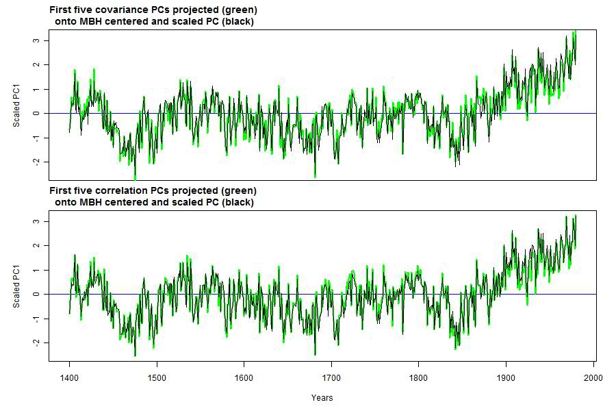
title("First five covariance PCs projected (green)
  onto MBH centered and scaled PC (black)",adj=0)

## Regress the covariance PCs against decentred
lm( scale(PCs[,1]) ~ PCs.3[,1:5] ) -> out
## Plot the resulting fitted curve
lines( tt, predict(out), col="green", lwd=2)
lines( tt, scale(PCs[,1])) ## ?? this just seems to replot the MBH PC1

## Same, but done for the correlation method
plot( tt,  scale(PCs[,1]),
type="l", lty=1, xaxt="n", ylab="Scaled PC1")
abline( h=0, col="blue")
title("First five correlation PCs projected (green)
  onto MBH centered and scaled PC (black)",adj=0)

lm( scale(PCs[,1]) ~ PCs.2[,1:5] ) -> out
lines( tt, predict(out), col="green", lwd=2)
lines( tt, scale(PCs[,1]))

par( oma=c(0,0,0,0), mar=c(5,5,2,2))
axis( 1)
mtext(side=1, line=3, text="Years")

}


Here's the plot:

I'll comment more on the results in the next post, and also look in more detail at the various PC's.