Update Correction to sensitivity to rotation below
Yet another post on this topic, which I have written a lot about. It is the the basis of calculation of global temperature anomaly, which I do every month with TempLS. I have developed three methods that I consider advanced, and I post averages using each here (click TempLS tab). They agree fairly well, and I think they are all satisfactory (and better than the alternatives in common use). The point of developing three was partly that they are based on different principles, and yet give concordant results. Since we don't have an exact solution to check against, that is the next best thing.
So why another one? Despite their good results, the methods have strong points and some imperfections. I would like a method that combines the virtues of the three, and sheds some faults. A bonus would be that it runs faster. I think I have that here. I'll call it the FEM method, since it makes more elaborate use of finite element ideas. I'll first briefly describe the existing methods and their pros and cons.
Mesh method
This has been my mainstay for about eight years. For each month an irregular triangular mesh (convex hull) is drawn connecting the stations that reported. The function formed by linear interpolation within each triangle is integrated. The good thing about the method is that it adapts well to varying coverage, giving the (near) best even where sparse. One bad thing is the different mesh for each month, which takes time to calculate (if needed) and is bulky to put online for graphics. The time isn't much; about an hour in full for GHCN V4, but I usually store geometry data for past months, which can reduce process time to a minute or so. But GHCN V4 is apt to introduce new stations, which messes up my storage.A significant point is that the mesh method isn't stochastic, even though the data is best thought of as having a random component. By that I mean that it doesn't explicitly try to integrate an estimated average, but relies o exact integration to average out. It does, generally, very well. But a stochastic method gives more control, and is alos more efficient.
Grid method with infill
Like most people, I started with a lat/lon grid, averaging station values within each cell, and then an area-weighted average of cells. This has a big problem with empty cells (no data) and so I developed infill schemes to estimate those from local dat. Here is an early description of a rather ad hoc method. Later I got more systematic about it, eventually solving a Laplace equation for empty cell regions, using data cells as boundary conditions.The method is good for averaging, and reasonably fast. It is stochastic, in the cell averaging step. But I see it now in finite element terms, and it uses a zero order representation within the cell (constant), with discontinuity at the boundary. In FEM, such an element would be scorned. We can do better. It is also not good for graphics.,
LOESS method
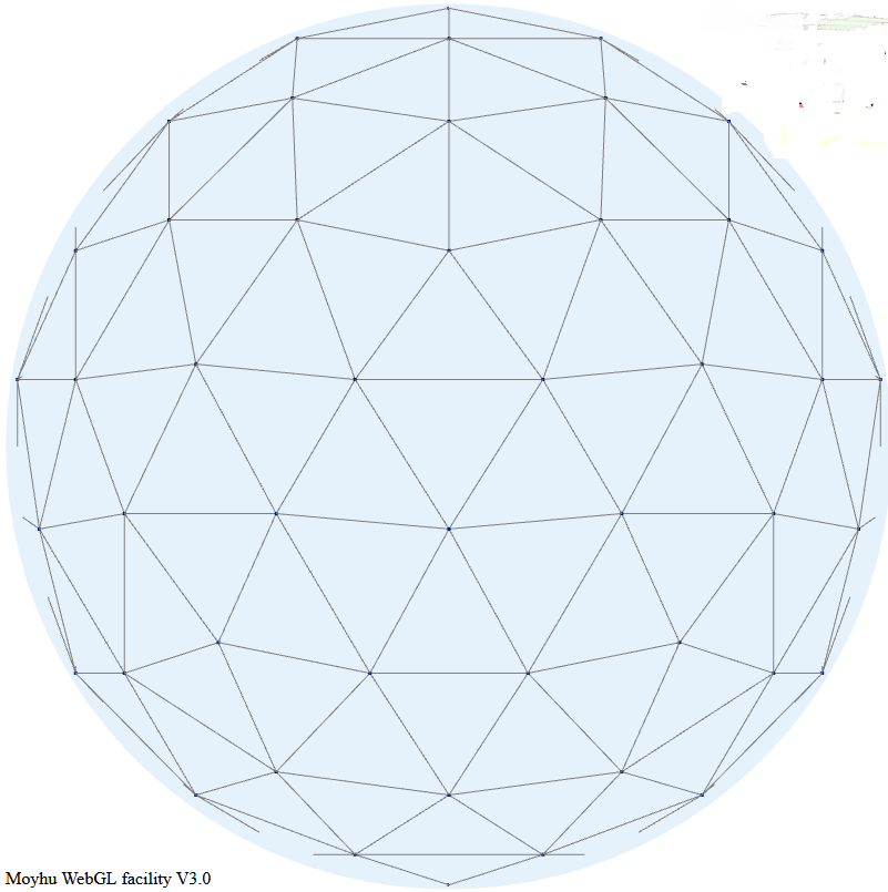
My third, and most recent method, is described here. It starts with a regular icosahedral grid of near uniform density. LOESS (local weighted linear regression) is used to assign values to the nodes of that grid, and an interpolation function (linear mesh) is created on that grid which is either integrated or used for graphics. It is accurate and gives the best graphics.Being LOESS, it is explicitly stochastic. I use an exponential weighting function derived from Hansen's spatial correlation decay, but a more relevant cut-off is that for each node I choose the nearest 20 points to average. There are some practical reasons for this. An odd side effect is that about a third of stations do not contribute; they are in dense regions where they don't make the nearest 20 of any node. This is in a situation of surfeit of information, but it seems a pity to not use their data in some way.
The new FEM method.
I take again a regular triangle grid based on subdividing the icosahedron (projected onto the sphere). Then I form polynomial basis functions of some order (called P1, P2 etc in the trade). These have generally a node for each function, of which there may be several per triangle element - the node arrangement within triangles are shown in a diagram below. The functions are "tent-like", and go to zero on the boundaries, unless the node is common to several elements, in which case it is zero on the boundary of that set of elements and beyond. They have the property of being one at the centre and zero at all other nodes, so if you have a function with values at the node, multiplying those by the basis functions and adding forms a polynomial interpolation of appropriate order, which can be integrated or graphed. Naturally, there is a WebGL visualisation of these shape functions; see at the end.The next step is somewhat nonstandard FEM. I use the basis functions as in LOESS. That is, I require that the interpolating will be a best least squares fit to the data at its scattered stations. This is again local regression. But the advantage over the above LOESS is that the basis functions have compact support. That is, you only have to regress, for each node, data within the elements of which the node is part.
Once that is done, the regression expressions are aggregated as in finite element assembly, to produce the equivalent of a mass matrix which has to be inverted. The matrix can be large but it is sparse (most element zero). It is also positive definite and well conditioned, so I can use a preconditioned conjugate gradient method to solve. This converges quickly.
Advantages of the method
- Speed - binning of nodes is fast compared to finding pairwise distances as in LOESS, and furthermore it can be done just once for the whole inventory. Solution is very fast.
- Graphics - the method explicitly creates an interpolation method.
- Convergence - you can look at varying subdivision (h) and polynomial order of basis (p). There is a powerful method in FEM of hp convergence, which says that if you improve h and p jointly on some way, you get much faster convergence than improving one with the other fixed.
Failure modes
The method eventually fails when elements don't have enough data to constrain the parameters (node values) that are being sought. This can happen either because the subdivision is too fine (near empty cells) or the order of fitting is too high for the available data. This is a similar problem to the empty cells in simple gridding, and there is a simple solution, which limits bad consequences, so missing data in one area won't mess up the whole integral. The specific fault is that the global matrix to be inverted becomes ill-conditioned (near-singular) so there are spurious modes from its null space that can grow. The answer is to add a matrix corresponding to a Laplacian, with a small multiplier. The effect of this is to say that where a region is unconstrained, a smoothness constraint is added. A light penalty is put on rapid change at the boundaries. This has little effect on the non-null space of the mass matrix, but means that the smoothness requirement becomes dominant where other constraints fail. This is analogous to the Laplace infilling I now do with the grid method.Comparisons and some results
I have posted comparisons of the various methods used with global time series above and others, most recently here. Soon I will do the same for these methods, but for now I just want to show how the hp-system converges. Here is the listing of global averages of anomalies calculated by the mesh method for February to July, 2019. I'll use the FEM hp notation, where h1 is the original icosahedron, and higher orders hn have each triangle divided into n², so h4 has 320 triangles. p represents polynomial order, so p1 is linear, p2 quadratic.
|
|
| ||||||||||||||||||||||||||||||||||||||||||||||||||||||||||||||||||||||||||||||||||||||||||
|
|
| ||||||||||||||||||||||||||||||||||||||||||||||||||||||||||||||||||||||||||||||||||||||||||
Note that h1p1 is the main outlier. But the best convergence is toward bottom right.
Sensitivity analysis
Update Correction - I made a programming error with the numbers that appeared here earlier. The new numbers are larger, making significant uncertainty in the third decimal place at best, and more for h1.
I did a test of how sensitive the result was to placement of the icosahedral mesh. For the three months May-July, I took the original placement of the icosahedron, with vertex at the N pole, and rotated about each axis successively by random angles. I did this 50 times, and computed the standard deviations of the results. Here they are, multiplied by a million:
|
|
| |||||||||||||||||||||||||||||||||||||||||||||||||||||||||||||||||||||||||||||||||||||||||||||
The error affects the third decimal place
Convergent plots
Here is a collection of plots for the various hp pairs in the table, for the month of July. The resolution goes from poor to quite good. But you don't need very high resolution for a global integral. Click the arrow buttons below to cycle through.Visualisation of shape functions
A shape functions is, within a triangle, the unique polynomial of appropriate order which take value 1 at their node, and zero at all other nodes. The arrangement of these nodes is shown below: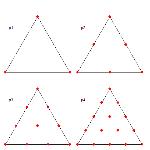
Here is a visualisation of some shape functions. Each is nonzero over just a few triangles in the icosahedron mesh. Vertex functions have a hexagon base, being the six triangles to which the vertex is common. Functions centered on a side have just the two adjacent triangles as base. Higher order elements also have internal functions over just the one triangle, which I haven't shown. The functions are zero in the mesh beyond their base, as shown with grey. The colors represent height above zero, so violet etc is usually negative.
It is the usual Moyhu WebGL plot, so you can drag with the mouse to move it about. The radio buttons allow you to vary the shape function in view, using the hnpn notation from above.


Hello Nick, you have posted inbetween so much info that it becomes hardly possible to recall where is what.
ReplyDeleteDo you have a corner where you post each month a few monthly time series (land-ocean, land, ocean) ?
That would be great help for folks who want to compare what they do with your more professional results!
Thx
J.-P. alias Bindidon
Bindidon,
DeleteOn the regular monthly data table, there is a button which switches to land/SST - that is HADSST etc and also .
You can also go to the active graph and choose just the datasets you want. Then the Data button will print out the data plotted in ascii.
Another option is to download a file
https://s3-us-west-1.amazonaws.com/www.moyhu.org/2019/10/month.sav
This is an R file with 28 data sets; the basis for the above presentations. Just change the 2019/10 to latest month. I keep copies like that so one can go back and see changes. I'll probably switch to csv format.
Thanks Nick but you misunderstood me I guess.
DeleteI of course did not mean the bunch of major data; that I have all already, including HadISST1, GHCN daily and others.
What I mean is a monthly time series
year month value
of what you produce each month (no: please no R files).
When I click on TempLSgrid
https://moyhu.blogspot.com/p/templsgrid.txt
or on TempLSmesh
https://moyhu.blogspot.com/p/templsmesh.txt
I obtain
"Sorry, the page you were looking for in this blog does not exist."
instead of a txt output...
Rgds
J.-P.
Bindidon,
DeleteYes, sorry, those files aren't working at the moment. But the data is in those tables. If you go to the head table on the data page, and click the TempLS tag, you'll get 8 different kinds of TempLS output back to start 2014. On the land/sst button, you'll get a further set of TempLS land and ocean. If you go to the active plot here, show TempLSmesh (or sst, land) and click the show data button bottom right, it will bring up a tab with data starting 1900.
I have put a file month.csv here. It has about 28 datasets back to 1850 (up to date). I'll keep doing that each month.
I am essentially using your MESH method, but recalculating the geometry for every monthly time step. It takes about 40mins to process all G4/HadSST3 from scratch which I think is not too bad. I also tried icosahedral grids but then simply averaged all values inside each cell to form an area weighted global average.
ReplyDeleteI am not sure I understand your LOESS method. In order to do a least squares fit you assume a polynomial distribution , but what are the dependent variables? Are they distance from a node point ? Do you only fit measurements inside one cell or what ?
Impressive though !
Thanks, Clive,
DeleteI have just put up a new post which sets out the maths more consistently. It also does comparisons. My mesh method took about an hour doing all meshing as new; the high resolution methods of FEM/LOESS (eg h4p4) take about five minutes.
The dependent variables are the multipliers of each shape function. There are a few underlying FEM tricks here. The basis functions are such that they are 1 on their node, and zero on all the other nodes. So f(z)=ΣaᵢBᵢ(z) is the unique element-wise polynomial which takes values aᵢ at the node locations zᵢ. It is also continuous. In the mesh method, these are the piecewise linear approximants.
So it is basically a regression to find which aᵢ bring f(z) to be least squares closest to the datapoints y. Then integrate f(z).
There are a whole lot of numbers for doing this which I can post if anyone is interested eg integrals of shape functions.