Global reconstructions with the new HADSST3
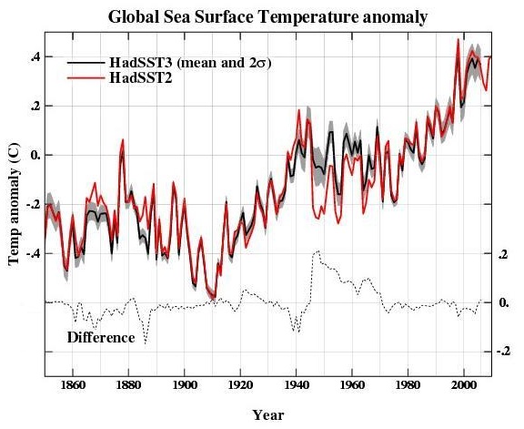
There is a new version of sea surface temperature records: HADSST3. It is reported here, commended here, and criticised here.The most noted change relative to HADSST2 is in a post-WW2 period when there was an issue with bucket and engine intake readings. HADSST2 was said to have a spurious dip in this period, which HADSST3 corrects. Consequently, trends of SST calculated over the last fifty years, say, have been slightly reduced.
I have not yet seen it used in any global land/sea index calculations. I have seen the effect inferred, but not measured.
Well, this is something TempLS V2.1 can do. So I downloaded HADSST3 from the Met Office site. Currently, it only goes as far as 2006. I compared it with using HADSST2, both in association with land measurements from GHCN v2.
Since the effect on trend has been a point of argument, I've made a plot of the trend calculated between 2006 (last year of HADSST3 currently) and years starting before about 1990, going back.
Update - I've added a table of trend values at the end of the post.
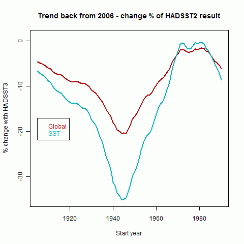
Update - since a lot of blog discussion talks of the % change in trend in using new HADSST3, I've replotted the last two plots of this post (qv) in % terms - change in the trend measured back from 2006, for both the SST average and for global land/sea. Here it is:
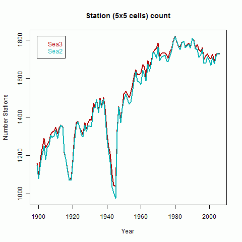
The output here is derived from the TempLS standard plots. The HADSST3 source was the HADSST3_median file. Firstly I show the "station" count. That is, the number of 5x5 cells in any year that have at least one monthly measurement. HADSST3 has more, but there is very little difference. The effects of the two world wars are obvious. In the legends "Sea3" or "SST3" refer to HADSST3, etc.
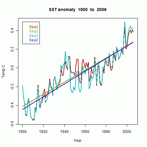
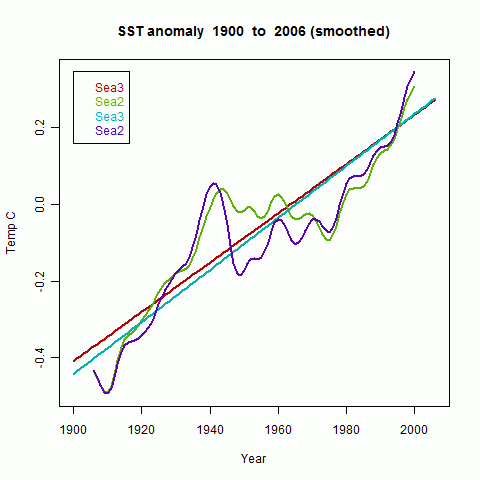
Next the area-weighted means of SST anomalies only, calculated with HADSST3 and HADSST2. As expected, HADSST3 substantially increases the average in the post-WW2 period. There's also a slightly puzzling discrepancy post-2000. ClimateAudit has a plot which is mostly similar, but doesn't have that discrepancy. (Update - I see that RealClimate shows a corresponding plot which does have this discrepancy). The least squares regression line is shown, and also a smoothed version:
|  |
Now comes the Global land/sea average, calculated using GHCN v2 means for land stations. The difference is similar, which is expected, since the SST measurements are a dominant component of the average.
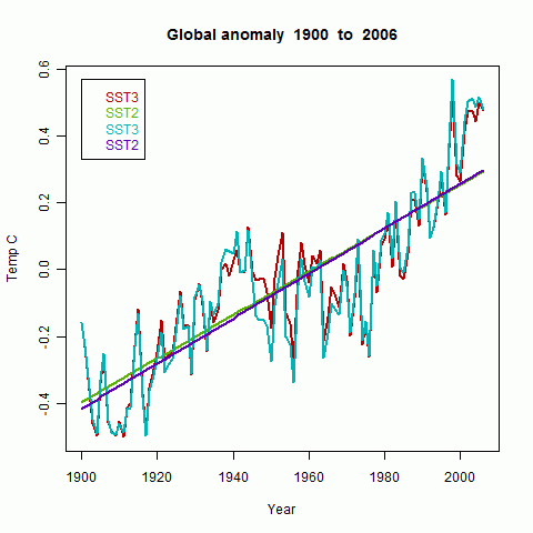
| 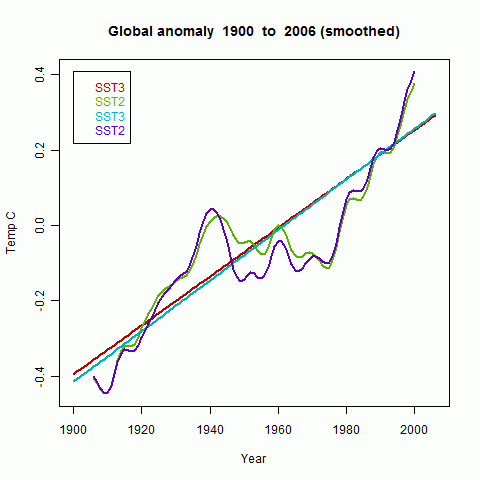 |
Here is an expanded version of each (unsmoothed) in the period 1950-2006:
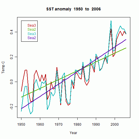
| 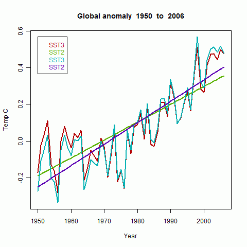 |
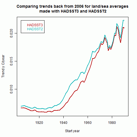
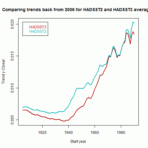
Finally, here is the trend of the global average, calculated back from 2006 to the year shown on the x-axis. As might be expected, there is a minor difference, greatest in the post WW2 years, but less before and after.
Update - for completeness, I've added the analogous plot for SST averages.
|  |
Update - here are the numerical trend values corresponding to the plots:
LamdSST2/3 are the global measures, Sea2/3 are the SST's. Standard errors do not allow for autocorrelation.
| Trend | LandSST3 | LandSST2 | Sea3 | Sea2 |
| 1900-2006 | 0.0649 | 0.06726 | 0.06425 | 0.0678 |
| Trend_se | 0.004124 | 0.00441 | 0.00359 | 0.003899 |
| 1950-2006 | 0.09755 | 0.1169 | 0.07075 | 0.09944 |
| Trend_se | 0.01056 | 0.01012 | 0.009047 | 0.008181 |


I think you have your legends muddled in every plot but the first. But it could be my colour vision.
ReplyDeleteKevin C
Kevin,
ReplyDeleteIt could be - my color vision isn't that great either. Abd the legend didn't spell out which was for the curve and which the corresponding regression line. I thought that would be fairly clear, but it isn't as good as I'd hoped.
Kevin,
ReplyDeleteThe confusion may be that the colors have inconsistent significance between unsmoothed and smoothed, say - I was using an automatic color scheme. I'll try to fix that.
Could you swap in GHCNv3 (which is no longer beta) and turn on your interpolation feature (assuming it works with SST)? I suspect that would give us the closest thing to "the truth" yet.
ReplyDeleteAlso, the post 2000 discrepency in HadSST2 actually begins in 1997 and is the result of some improperly merged data. When you difference HadSST2 with any other dataset, there is a step change that coincides exactly when Hadley switches to a different data source.
CCE,
ReplyDeleteYes, I'll do that. For the first post, I wanted to make sure that anything unfamiliar could be attributed to HADSST3 rathet than another new dataset. Somewhat for the same reason, I didn't try to go back beyond 1900. I'll do a post with those covered.
"The most noted change relative to HADSST2 is in a post-WW2 period when there was an issue with bucket and engine intake readings. HADSST2 was said to have a spurious dip in this period, which HADSST3 corrects."
ReplyDeleteSaying this has been "corrected" may be a little optimistic. What has been done is that the step change had been abandoned and replaced with a similar change, that is phased in over about 30 years.
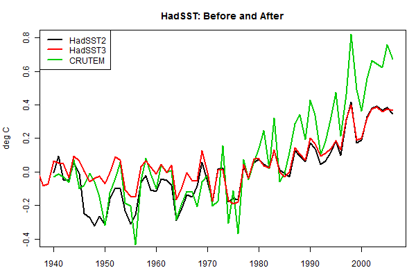
Here are the adjustments of HadSST2 and HadSST3 compared:
http://curryja.files.wordpress.com/2012/03/hadsst-icoads1.png
There is a detailed examination of the issues behind these adjustments and their effects on the data over at Judith Curry's site.
judithcurry.com/2012/03/15/on-the-adjustments-to-the-hadsst3-data-set-2
There is also an interesting discussion with Met Office's John Kennedy in the comments. Search for his name using browser , since there are a lot of comments.
He gives some useful insight into how the data is processed.
In essence the 0.5 degree drop is still there , it's just been smoothed out so it is not so obviously wrong. Whether that makes it "right" is debatable.