Lisbon Meeting

My last post said that I would be away - the main object of my travel was to attend the Lisbon Workshop on Reconciliation in the Climate Change Debate. For an excellent summary of the meeting, and its background and purposes, I recommend Judith Curry's two threads (Part I and Part II ). The discussion is interesting too - other participants chime in.

WUWT also has several threads (here too) and has posted the organisers' statement of purpose. Other atttenders have blogged - Tallbloke, Steven Goddard.

I won't at this stage try to add to the facts of what Judith has said. My assessment was similar too. I was interested in Jerome Ravetz' ideas, and impressed by his guidance of the meeting. But I don't have much to say about postnormal science, which I regard as being about society rather than science.

I am very glad I attended the meeting, to hear and meet the participants. I think an agreed outcome was always unlikely, so I was not disappointed there.

I will be travelling for another few days, so apologies in advance if my responses are sometimes delayed.

Update - Deep Climate asked for the list of participants. Here it is, as circulated at the meeting:

Jerome Ravetz	James Martin Institute, Oxford Univ., UK
James Risbey	CSIRO, AUS
Jeroen van der Sluijs	Univ. Utrecht, NL
Alice Benessia	Univ. Torino, IT
Tom Boersen	Aalborg University Copenhagen, DK
Judith Curry	School of Earth and Atmospheric Sciences, Ga Institute of Technology, Atlanta, GE, USA
Steve Goddard	Science and Public Policy Inst., VA, USA
Sofia Guedes Vaz	New Univ. of Lisbon, PT
Bill Hartree	UK Measurement Institute, UK
Werner Krauss	Center for Mediterranean Studies, Bochum, DE
Steve McIntyre	Climate Audit, CAN
Ross McKitrick	Department of Economics - University of Guelph, CAN
Jean-Paul Malingreau	European Commission – Joint Research Centre
Steve Mosher	Independent consultant, USA
Ana Lopez	London School of Economics, UK
Fred Pearce	The Guardian, UK
Tiago Pedrosa	New Univ. of Lisbon, PT
Roger Tattersall	Leeds Univ., UK
Gerald Traufetter	Spiegel, DE
Louise Romain	The Center for Nonviolent Communication
Viriato Soromenho Marques	Univ. of Lisbon, PT
Nick Stokes	CSIRO, AUS
Peter Webster	School of Earth and Atmospheric Sciences, Georgia Institute of Technology, Atlanta, GE, USA
Hans Von Storch	Meteorological Institute, Univ. Of Hamburg
Ângela Guimarães Pereira	European Commission – Joint Research Centre
Silvio Funtowicz	European Commission – Joint Research Centre
Ines Crespo	European Commission – Joint Research Centre
Paula Curvelo	European Commission – Joint Research Centre

A JS gadget for viewing temperature trends.

In my previous post I showed a map of all possible trends calculated over sub-time intervals of a period, with a mechanism for selecting different datasets and periods. Since there seem to be ongoing interest in viewing trends, I thought a useful Javascript gadget could be developed from that.

Now when you select a dataset/time combination, a corresponding time series plot is displayed, with two colored balls representing the start and end of each trend period. The numerical data are displayed on the right. There are several ways of controlling the horizontal position of the balls:

• You can click on the colored triangle. Each position represents a start/end combination, so the balls will move to the endpoints of the fitted regression line, and the slope and locations will appear on the right. It's a realisation of the color on the plot, and should correspond.
• You can move the balls by clicking on the red or blue bars on the graph.
• You can nudge, for fine control, using the <<<<>>>> device of the appropriate color. The outside symbols move the ball of that color by 8 months, the next by 4 and the innermost by 1.

Hadcrut is in - final temperature summary for 2010

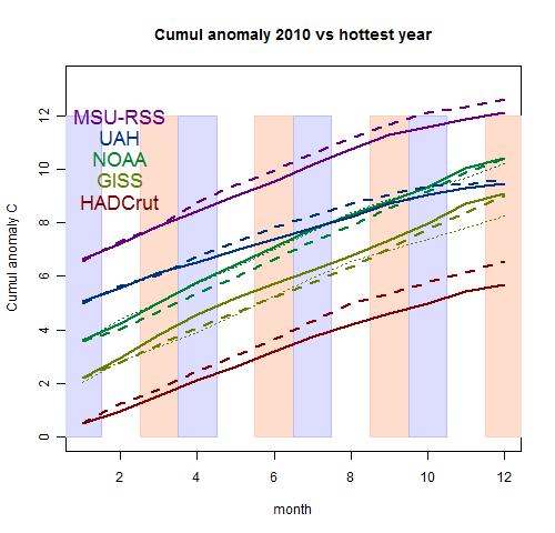
Hadcrut reported a 0.251°C mean NH/SH anomaly for December, down from 0.455°C in Nov. As expected, that leaves 2010 well behind 1998 in Hadcrut's record (about 0.1°C less).

So in summary, the indices that had 1998 as hottest (Hadcrut, UAH, MSU) keep it there (UAH was close). Those that had 2005 as hottest (GISS, NOAA) say 2010 was about the same.

I guess I'll run a tracking plot for 2010, but won't start until a few months into the year. I normally update it on this post, but since it's the final for 2010, I'll show it below:

On "Mannian" Smoothing

A recent thread at Climate Audit revisited the topic of "Mannian" smoothing. There's a long history here - here, for example, is a thread to which this seems to be a sequel.

The "Mannian" smoothing to which they refer is described, under the name of Minimum Roughness Criterion, by Mann GRL04 (2004), with a follow-up GRL08.

There was much more discussion of the general idea of Mannian smoothing in some threads on its use by Rahmstorf; at CA: the-secret-of-the-rahmstorf-non-linear-trend
and rahmstorf-et-al-reject-ipcc-procedure, and at Lucia's: more-fishy-how-doesdid-mann-guess-future-data-to-test-projections


In this post I'll try to describe what "Mannian" smoothing does, and why, and how it compares with other methods in the statistical literature.

Smoothing and the endpoint problem

Smoothing time series data (y_t) is often done using a symmetric digital filter on a finite base:
Y_t=a₀y_t+Σa_k(y_t-k+y_t+k)
summed over the M coefficients (or weights) a_k, k=1:M
Symmetric is favored because the result is centred - ie the weighted average that it produces represents the value at the centre of the weighting - no lag. If you apply it to straight line data, it returns the line unchanged.

But at each end of the data, you run out of points. You could stop the smoothing as soon as this happens. But that seems excessive - the quality of the smooth will degrade as you approach the endpoints, but it does not immediately become worthless. And sometimes the most recent data is where you really want to know the best estimate of trend, even if it is unstable and likely to change as new data arrives.

This is not a new problem, of course. Alastair Gray and Peter Thomson wrote several papers in mid 1990's in which they sought filters which would require minimum revision as new data came in. In the process they reviewed the history of one logical way to achieve that, which was to use some forecast based on existing data to "pad" the data so a symmetric filter could be used. I'll say more on the legitimacy of that, but here's what they said about its history:

A common and natural approach involves forecasting the missing values, either implicitly or explicitly, and then applying the desired central filter. The forecasting methods used range from simple extrapolation to model based methods, some based on the local trend model adopted, others based on global models for the series as a whole. The latter include the fitting of ARIMA models to produce forecasts (see Dagum (1980) in particular). The principle of using prediction at the ends of series seems a key one which goes back to DeForest (1877). See also the discussion in Cleveland (1983), Greville (1979) and Wallis (1983).

Mann's papers and method

In GRL04 Mann describes three boundary conditions that one could try to meet by extrapolating:

1. Minimum norm - ie deviation from some target value, usually a known value ("climatology").
2. Minimum slope - the final slope should be zero. This allows the smooth more freedom to shape itself to the end data, but is no use if you want an estimate of the end slope, because that has been prescribed (zero).
3. Minimum roughness - the second derivative should be zero. This allows an estimate of both the final value and slope. It's the least intrusive of the three, in that the second derivative is hardest to estimate accurately, so prescribing it gives least loss of information.

If the smoother operates over 2M+1 points, then M points must be padded at each end. The conditions themselves do not uniquely a padding formula - M glides over this a bit to go straight to formulae which will do the job. They are:

1. Minimum norm - pad with the constant "longterm mean".
2. Minimum slope - reflect the M values preceding final t value about that t - ie the extension makes the series symmetric (even) about the endpoint. 
3. Minimum roughness - reflect the same M values about both the final t and final y, so the series makes an odd function about that point. This means any fitted model will have zero second derivative (and all even higher derivatives).

Mann showed this plot of the effect of the three methods on the annual mean NH temperature series:

The smoother is a Butterworth filter. Note that the min norm deviates most, and is a poor fit near trhe end. The measure of fit is MSE - the ratio of variance of residuals from the smooth vs variance about the mean.

It is important to remember that although Mann's methods invoke a forecast, or symmetry, when you combine the linear forecast formula with the symmetric filter, you end up with an unsymmetric filter on the known data set.

Pegging the endpoint and centering

A necessary feature of the minimum roughness method is that the smooth passes through the final point - "pegged" to it. This has also been a source of criticism - in fact the most recent CA thread seems to focus on it.

It is indeed a clear acknowledgement that the effectiveness of the smoothing has failed right at the end. But something does have to give there. At least the final estimate is unbiased. It will be subject to perhaps more vigorous change as new data comes in than, say, the Gray/Thomson value. But that is not a huge problem.

A virtue of the Mann method is that it is automatically centered. That is, the weighted average used for the smooth is indeed appropriate for the centre value. There isn't a lag. A test of this is whether a line would be returned unchanged. One would hope so. This is not just an issue of "prettiness"; the point of a filter is that it should shake off the noise and return the underlying process, and if it shifts even a line, then it will shift any trend you are using it to find.

It is also desirable, generally, to use positive weights. If the symmetric filter is positive, then so will be the modified weights as you approach the end. And it is then easy to show that if you have centred, positive, possibly asymmetric filter at the final point, that filter must reduce to a one-point one - ie, pegging.

Comparison with a method used in economic statistics.

There was an undercurrent of scepticism about the use of forecast values. Lucia was especially vehement. But it is a well established technique, as the above quote from Gray et al showed. In fact smoothing and forecasting are closely related. Both rely on some model (eg polynomial) fitted to the data, and if you use the model to generate forecast values which are then used to calculate coefficients, then there is no extra assumption.

Mann doesn't quite do that - he uses a symmetry property of the underlying model. Suppose you were forming the smoother by polynomial fitting. The "forecast" for minimum roughness is then just a constraint that the polynomials use odd powers of t (with the t origin at the final endpoint).

The most explicit formulation of a method with forecasting seems to have been a technical report by Musgrave (Musgrave, J. C. (1964). A set of end weights to end all end weights. Working paper, Bureau of the Census, US Department of Commerce, Washington, D.C.). This wasn't published, and doesn't seem to be online, but it has been frequently cited. It is summarised in this 2003 paper by Quenneville et al. Unfortunately, I couldn't find a free version. It invokes the Henderson smoother, which is popular with census folk, and common in economics. In fact, the 25-point Henderson filter with Musgrave end smoothing makes up the widely used X-11 smoothing (or seasonal adjustment) procedure.

The Musgrave endpoint process works thus (Quenneville). With a symmetric filter, for each point where there are insufficient data points:

1. Fit a OLS reegression y = a + b*t to the points that are available
2. Pad the data with the line y=a+b*t+g*b*(t-mean(t))
   where g=var(b)/(b^2+var(b)) and the mean is over the needed padding interval
3. apply the symmetric filter to the region with padding

Note that different padding is used for each smooth point.  The modified line for extrapolation, with the factor g, ensures that the expected adjustment for new data is minimised, rather than SS residuals.

Examples

The code for these examples is called mauna.r, at the Document Store

I'll calculate first a data set where there is a clear linear trend. This is the set of annual average CO2 readings at Mauna Loa. I'll use the AR4 13-point filter, as referenced here. It's similar to a binomial filter, and they used it with minimum slope, describing this as a conservative option. Here are the last few years, showing minimum slope, Mannian and Musgrave endpoint smoothing.


Note that in this case minimum slope is the one out of line. The attempt to make the end slope zero is just inappropriate, and it shows. The fault is even clearer is I superimpose the results that you would have got starting in 2008, and then updating as each years data come in. Not only does minimum slope deviate, but it needs a bigg correction each year,

Now, for something less regular. Here are the NOAA monthly global temperature anomalies. First the most recent plot:

This shows more clearly how Mannian (MRC) pegs to the endpoint, so there is no smoothing there. Musgrave seems to do better. Minimum slope looks better here, mainly because the slope is indeed closer to zero.

Now here is the same plot with three successive months superimposed, as if we had started in October, then plotted for November and December. Now minimum slope looks good, but again, only because there isn't much slope. Musgrave oscillates a bit more, and Mannian much more, because of the pegging.

Conclusion

Firstly, there's nothing wrong in principle with Mannian smoothing. The padding process is similar to the widely used Musgrave method, and it doesn't seem to show any particular bias. But the pegging to the endpoint value does make for greater variation.

Minimum slope is, as the AR4 said, more conservative. But it pushes for a zero end slope when that may be clearly inappropriate.

I think the Musgrave process, which does explicitly seem to minimise adjustment on new data, is probably the best choice.

The code for these examples is called mauna.r, at the Document Store .

GISS shows 2010 as record hot for land/ocean - NOAA declares tie with 2005.

The GISS index for December is out, and while at 0.4C the anomaly is much less than November, it was still just enough to beat 2005. I have updated the tracking plot.

The NOAA also say that 2010 tied with 2005 as hottest year, but don't give the actual anomalies. It isn't in their usual data file, so I can't plot it.



Roy Spencer has the UAH Dec figure, down 0.09C on November. But he's using a new adjustment period, so I haven't figured how to update the existing graph. It probably won't be hard, but Ive been waiting for them to update the existing data file. Maybe it's obsolete. Anyway, it would have required a very big increase to reach a record level here.

Update.  GISS describes the result as a "statistical" tie between 2005 and 2010. The NOAA number is posted now, and 2010, if you average monthly means, fell just behind 2005. Very close.

Anomaly °C	GISS	NOAA
2010	0.6325	0.6169
2005	0.6242	0.6183
1998	0.5642	0.5984

From the climate point of view, it really doesn't matter which was hottest. 2010 was just another of the recent warm years.

Update. Zeke has pointed me to a more up-to-date UAH data set. So I've added that to the plot - it didn't make any records. The tracker plot (for UAH) looks different because of the new baseline - in fact it sags over the next plot below. But since this is nearly the last plot for 2010, I didn't move it.

RSS posts December average - 2010 lagged 1998.

RSS posted its December average, and confirmed what had been expected for 2010 - short of the record average in 1998, but still second hottest.  I've updated the tracking plot.

GISS looks likely to report 2010 as the hottest year recorded. NOAA is less clearcut, but still quite likely. The other indices are likely to maintain 1998 as hottest.

I'll be mostly offline for a few days - back at the weekend.

On greenhouses and the Greenhouse Effect

From time to time, some people get excited about the fact that the greenhouse effect seems wrongly named. An extreme case is the paper of Gerlich and Tscheuschner, where they devote a whole section 2 (19 pages) to the question. It continues to arise; Judith Curry touched on it in a recent thread, where discussion turned to the old Wood's experiment

The standard response correctly says that none of this matters. The atmospheric  GHE is what it is, and is no less true if it turns out that the allusion to greenhouses is inaccurate. Wikipedia takes this approach, with a refreshing brevity and directness.

However, there is a little more to the story (which still says nothing about the truth of the GHE). Greenhouses do work mainly by blocking heat loss through convection. But IR flux blocking is not totally insignificant.

Wood's experiment

The description of this in the 1909 Philosophical Magazine is indeed brief. Some people give the impression that he built a greenhouse out of rock salt, but the geometry seems to be simpler and on a much smaller scale. Still, he concluded:
It seems to me very doubtful if the atmosphere is warmed to any great extent by absorbing the radiation from the ground, even under the most favourable conditions.

This final statement is little emphasised, but seems to be amply justified by the sketchiness of the note:
I do not pretend to have gone very deeply into the matter, and publish this note merely to draw attention to the fact that trapped radiation appears to play but a very small part in the actual cases with which we are familiar.

Indeed he didn't.

Modern Greenhouses

Ironically, the situation that forced Wood to use rock salt as an IR-permeable material is now reversed. In his day, greenhouses were always made of IR-blocking glass. Now they are often made of IR-permeable plastic. And, in support of Wood, they do work. They block convective heat transport, and also provide an insulating effect to limit conduction through the boundary.

However, a moderate amount of heat is still transferred by IR. Ironically, a reason why it isn't larger on balance is because of the countervailing downwelling IR, also a subject of occasional skepticism. Downwelling IR, from the atmosphere and especially clouds, is not that much less than upwelling. Glass blocks both upwelling and downwelling; the nett flux blocking is small, but if you are focussing on the fate of heat emanating from the surface, the IR fraction that is blocked us a larger fraction.

A real greenhouse issue

A covering that blocks IR actually makes a real improvement to greenhouse efficiency. It is more expensive, and people are willing to pay for it. Here are some industry observations:
NSW Ag Dept:
For example, films may be used to exclude ultra violet (UV) light for chemical free pest control or reflect long wave infra red (IR) radiation to improve heat retention at night. ... Long wave radiation (2500-40000 nm) absorbers reduce the loss of heat radiated from materials and objects (including plants) inside the greenhouse.

Or this advice
You can also buy a plastic film with an infrared inhibitor; it cuts heat loss inside the greenhouse by up to 20% on a cloudless night.
Actually, it would also cut loss on a clear day.

And here is a pamphlet which describes the practicality in some detail (for heated greenhouses, but the principle is the same).
The IR / anti-condensation treated films cost about $0.015 per square foot more than untreated films but reduce energy use by 15 to 20%.

Scale Issues

The main thing wrong with the Wood's style reasoning is scale. IR blocking is a minor effect on the scale of a greenhouse because convection is relatively much more effective. The temperature gradients are huge compared to what is maintained in the atmosphere. Wood compounded this by experimenting on a much smaller scale again.

In the atmosphere, IR transport is more important than convection, so the blocking effect of GHG's matters much more.

.