This was intended as a graphic facility for my post on GHCN data. However, alas, there was mission creep, and a dynamic trend viewer, in the style of the trend viewer page, emerged. It's "dynamic" because it is all in Javascript. I don't have to pre-calculate and store images. This is fine for annual data - calc time might be a problem for monthly. But the style of access also gives a rapid response which is fun to play with.
As with the trend page, I show a graph of the time series. Data options supplied are the usual collection of global temperatures, but you can also supply your own. And there is a color triangle, in which each dot (square) is a start/end year combination, with the color showing the corresponding trend. With the trend page, you could click on that to change the range; there were also controls in the graph. Now you just run the mouse over the triangle, and the red trend line on the plot moves dynamically, and the information is echoed top right. The triangle is oriented so the NE corner is starting ending 2014, and SE is the whole range. x axis is start year, y-axis is end year. The info in the upper triangle will tell you where you are.
I haven't given a color key, because you get an instant print response - basically, rainbow with red for warming. To change data set, select from the menu and then press the "Enter data" button. To enter your own, just convert it to a comma separated one-line list, and paste into the text window, and then click "Enter Data". The button enters the last thing you changed (text window or selector). If you enter data, it is attached to the choice "User Data" in the data menu. Initially, I have put a sinusoid there, which you can select. It shows graphically how the trend works as a derivative.
So here is the gadget:
The CI's are, like the trend page, calculated as AR(1) autocorrelated series using the Quenouille approx. Usually correlation is less for annual data. I have shown trends of all lengths, but too short trends will have unreliable or NaN CI's.
Tuesday, April 7, 2015

Wednesday, April 1, 2015
Early note on March 2015 global
Most of the NCEP data for March global surface temperature is in, and despite some cooling at the end, it still looks to be a little warmer than February. Probably less than May 2014, but higher than any other month in 2014 (or 2015). I'd expect this to be reflected in surface temps.
I've fixed a bug where in the daily NCEP table, dates were written one day ahead (on Australian time). Dates on the maps were correct.
I've fixed a bug where in the daily NCEP table, dates were written one day ahead (on Australian time). Dates on the maps were correct.
Thursday, March 26, 2015
GHCN Monthly data portal
I am planning to add station data to the GHCN V3 monthly portal. Not monthly data which would be cumbersome, but annual average. This is useful for plotting and trends.
There is a trial below. Each link leads to the NOAA GHCN station summary, as before, but the radio button brings up a page with a table of the annual averages, along with a brief metadata and a map (the station is in the middle). There is a table for unadjusted data, and below for adjusted. Both are then repeated in CVS format, for import into Excel. The table of links is searchable (Ctrl-F), and can take a while to load. I'll probably add a graphing and trend calculation capability.
In calculating the annual averages, I eliminated years with less than 9 months data. I also (before) removed data with flags indicating unreliability. Then I infilled missing months with the overall mean for that station/month (else seasonal effects add a lot of noise). Then I calculated the simple average of the infilled data.
There is a trial below. Each link leads to the NOAA GHCN station summary, as before, but the radio button brings up a page with a table of the annual averages, along with a brief metadata and a map (the station is in the middle). There is a table for unadjusted data, and below for adjusted. Both are then repeated in CVS format, for import into Excel. The table of links is searchable (Ctrl-F), and can take a while to load. I'll probably add a graphing and trend calculation capability.
In calculating the annual averages, I eliminated years with less than 9 months data. I also (before) removed data with flags indicating unreliability. Then I infilled missing months with the overall mean for that station/month (else seasonal effects add a lot of noise). Then I calculated the simple average of the infilled data.
Friday, March 20, 2015
Central Australian warming
I've been arguing again, at Climate Etc. Blogger Euan Mearns has a guest post in which he claims to demonstrate that stations within 1000km of Alice Springs show no warming.
I'll post about it here, because it illustrates the averaging fallacies I've been writing about regarding Steven Goddard and colleagues (also here). And also because "Alice Springs" is one of those words naysayers sometimes throw at you as if no further explanation is required (like Reykjavik). People who do that generally don't know what they are talking about, but I'm curious, since I've been there.
There are actually two issues - the familiar time series of averages of a varying set of stations, and anomalies not using a common time base. I'll discuss both.
The stations are obtained from the GISS site. If you bring up Alice Springs, it will indicate other stations within a radius of 1000 km. My list was 29, after removing repetitions. I've given here a list of the stations, together with the calculated trends (°C/century) and the long term normals. For all calculations I have used annual averages, discarding years with fewer than nine months data. The annual data (unadjusted GHCN V3 monthly from here) that I used is in CSV form here.
So Euan's post shows a time series of whetever reported in each year:

And, sure enough, not much trend. But he also showed (in comments) the number of stations reporting

Now what his average is really mainly showing is whether that highly variable set has, from year to year, hotter or colder locations. To show that, as usual I plot the same averaging process applied to just the station normals. This has no weather aspect:
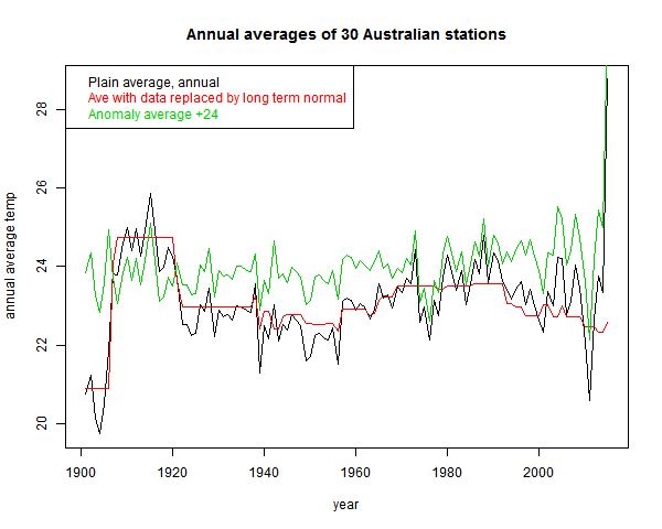
You see the red curve. That incorporates much of the signal that the fallacious black curve includes.
The effect is not as severe as Goddard's, because the stations are more homogeneous. The range of normal variation is less. It can be reduced, of course, by subtracting the mean. That is the green "anomaly" plot that I've shown. It is more regular, but still not much trend. That brings up the anomaly fallacy.
This is the fault of comparing anomalies using varying base intervals. I've described it in some detail here. If the stations have widely different periods of data, then the normals themselves incorporate some of the trend. And subtraction removes it.
This is a well-known problem, addressed by methods like "common anomaly method" (Jones), "reference stations method" (GISS), "first difference method" (NOAA). I mention these just to say that it is a real problem that major efforts have been made to overcome.
As a quick and mostly OK fix, I recommend using regression fits for a common year, as described here. But the more complete method is a combined regression as used in TempLS (details here)
Update - to be more specific, as in the link it is best to do this in conjunction with some scheme for preferring data local to a region. There I used weighting. But to stick closest to the convention of using a fixed interval like 1961-90, my process would be:
1. If there is enough data in that interval (say 80%) use the regression mean over the interval
2. If not, then extend the interval to the minimum extent necessary to get 30 (or 24) years of data.
So I've done a combined regression average:
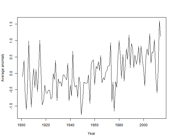
It's clearly warming since about 1940. And by about a degree.
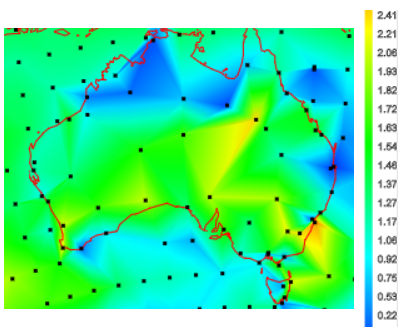
The station trends over their observed periods are almost all positive. So they are over a fixed period. Here, from the active trend map is a snap of trends in Australia since 1967:
Plots of the station data are somewhat obscured by noise. From Climate Etc:

It is rising. But a modest degree of smoothing - a 9 point triangular filter, gives:
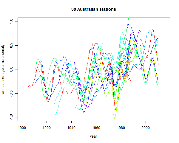
The uptrend is now unmistakeable.
I'll post about it here, because it illustrates the averaging fallacies I've been writing about regarding Steven Goddard and colleagues (also here). And also because "Alice Springs" is one of those words naysayers sometimes throw at you as if no further explanation is required (like Reykjavik). People who do that generally don't know what they are talking about, but I'm curious, since I've been there.
There are actually two issues - the familiar time series of averages of a varying set of stations, and anomalies not using a common time base. I'll discuss both.
The stations are obtained from the GISS site. If you bring up Alice Springs, it will indicate other stations within a radius of 1000 km. My list was 29, after removing repetitions. I've given here a list of the stations, together with the calculated trends (°C/century) and the long term normals. For all calculations I have used annual averages, discarding years with fewer than nine months data. The annual data (unadjusted GHCN V3 monthly from here) that I used is in CSV form here.
The Goddard Fallacy
So Euan's post shows a time series of whetever reported in each year:
And, sure enough, not much trend. But he also showed (in comments) the number of stations reporting
Now what his average is really mainly showing is whether that highly variable set has, from year to year, hotter or colder locations. To show that, as usual I plot the same averaging process applied to just the station normals. This has no weather aspect:
You see the red curve. That incorporates much of the signal that the fallacious black curve includes.
The effect is not as severe as Goddard's, because the stations are more homogeneous. The range of normal variation is less. It can be reduced, of course, by subtracting the mean. That is the green "anomaly" plot that I've shown. It is more regular, but still not much trend. That brings up the anomaly fallacy.
The anomaly fallacy
This is the fault of comparing anomalies using varying base intervals. I've described it in some detail here. If the stations have widely different periods of data, then the normals themselves incorporate some of the trend. And subtraction removes it.
This is a well-known problem, addressed by methods like "common anomaly method" (Jones), "reference stations method" (GISS), "first difference method" (NOAA). I mention these just to say that it is a real problem that major efforts have been made to overcome.
As a quick and mostly OK fix, I recommend using regression fits for a common year, as described here. But the more complete method is a combined regression as used in TempLS (details here)
Update - to be more specific, as in the link it is best to do this in conjunction with some scheme for preferring data local to a region. There I used weighting. But to stick closest to the convention of using a fixed interval like 1961-90, my process would be:
1. If there is enough data in that interval (say 80%) use the regression mean over the interval
2. If not, then extend the interval to the minimum extent necessary to get 30 (or 24) years of data.
The anomaly fix
So I've done a combined regression average:
It's clearly warming since about 1940. And by about a degree.
Other evidence of warming
The station trends over their observed periods are almost all positive. So they are over a fixed period. Here, from the active trend map is a snap of trends in Australia since 1967:
Plots of the station data are somewhat obscured by noise. From Climate Etc:
It is rising. But a modest degree of smoothing - a 9 point triangular filter, gives:
The uptrend is now unmistakeable.
Tuesday, March 17, 2015
February GISS up 0.04°C
late news, but I've already posted twice on February temp. This is the regular post comparing GISS with TempLS.
GISS rose from 0.75°C in Jan to 0.79°C as predicted by Olof and JCH. TempLS also rose by a small amount. Troposphere measures showed a small decline.
Here is the GISS map. As with TempLS, very strong features - Russia and N Europe warm, East N America cold, and the West warm. Also a warm spot in Sudan - I had thought it might be a TempLS artefact.

And here is the corresponding TempLS map, as on St Patrick's Day:

GISS rose from 0.75°C in Jan to 0.79°C as predicted by Olof and JCH. TempLS also rose by a small amount. Troposphere measures showed a small decline.
Here is the GISS map. As with TempLS, very strong features - Russia and N Europe warm, East N America cold, and the West warm. Also a warm spot in Sudan - I had thought it might be a TempLS artefact.
And here is the corresponding TempLS map, as on St Patrick's Day:
Friday, March 13, 2015
February TempLS was warm
China GHCN data was late, but is now in (report here). The global average temperature was 0.694°C, slightly up from Jan 0.674. A small rise, but January had already tied May 2014, which was the hottest month of last year. So it's a warm start to 2015. The last month warmer than Feb was Nov 2013.
The map is pretty simple. A big warm band across Russia and NE Europe. Cold in E N America, but warm in the W and Akaska.
The map is pretty simple. A big warm band across Russia and NE Europe. Cold in E N America, but warm in the W and Akaska.
Tuesday, March 10, 2015
Derivatives and regression again
I've been writing about how a "sliding" trend may function as a estimate of derivative (and what might be better) here, here, here and here. There has been discussion, particularly commenter Greg. This post just catches up on some things that arose.
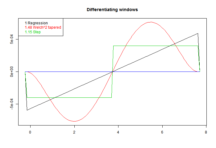
These are scaled to give correct derivative for a line. On the legend, I have written beside each the RMS value. Sqrt of the integral of square. That's the factor that you would expect to multiply white noise, as a variance of weighted sum. Ordinary regression has the least value. That is an aspect of its optimal quality. Better smoothing for HF comes at a cost.
So now to apply these to a sinusoid. In the following plot the yellow is the sine to be differentiated, the continuous curve "Deriv" is the exact derivative, and I have applied the three windows with three different footprints (line types). At each end, a region equal to half a footprint is lost - I have marked those parts with a horizontal line, which tells you how long each footprint was.
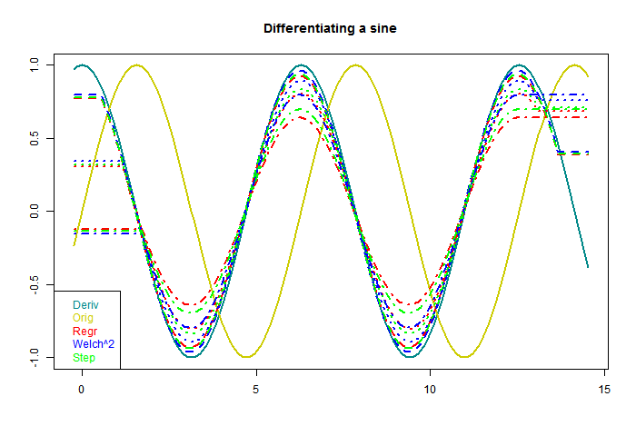
The first thing to note is that each gives a sinusoid, with the correct 90° phase shift. The is a consequence of being an odd function. Second is that as the footprint broadens, the amplitude shrinks. The inaccuracy is because a wider footprint is more affected by higher derivatives of the sine. In effect, it smoothes the result, to no good purpose here. But when there is noise, the smoothing is needed. That is the basic trade-off that we will encounter.
You'll notice, too, that both the Welch and step do better than regression. This is basically because they are weighted to favor central values, rather than any more subtle merit.
Now for something different, to differentiate white noise. There should be no real trend. I've dropped the step filter. Again the horizontal end sections indicate the half-footprint.
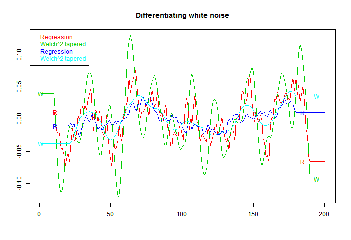
Now what shows is a marked oscillation, with period about equal to the footprint. The Welch filter is good at damping frequencies beyond this range; however, the actual amplitude of the response is much higher. That is associated with the higher RMS value noted on the first figure, and is commensurate with it.
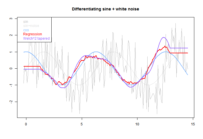
The pale grey is the original, sine and total. The blue is the derivative of sine. The red OLS regression tracks better than the smoother purple, but has more residual HF. Again the half-footprint is shown by the level sections at each end.
A way to do this is to take a family of windows, and make them orthogonal to higher powers by Gram-Schmidt orthogonalisation. I did that using OLS, OLS with Welch taper, and OLS with Welch^2 (W0,W1,W0). Here are the resulting windows. W1 is guaranteed to be accurate for a cubic, and W2 for fifth order:
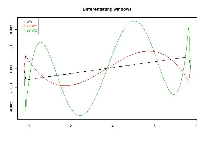
Again, they are scaled to give the same derivative. We see a more extreme version of the RMS inflation of the first fig. The higher order accuracy is got at a cost of much larger coefficients. They do indeed differentiate better, as the next plot shows:
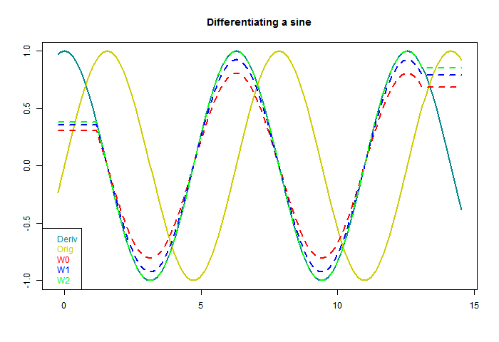
W2 seems suspiciously perfect. But each result is just the correct sinusoid multiplied by a scalar, and I think it just approaches 1 in an oscillatory way, so W2 just happens to be a zero. Anyway, here higher order certainly works. What about with white noise?
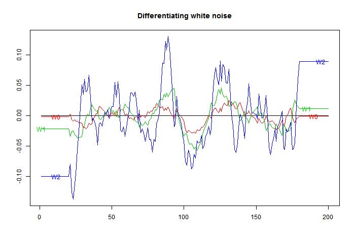
Here is the downside. The higher orders amplify noise, in line with their RMS integrals.
Higher order may sometimes work. If you have an exact cubic, then you can expand the footprint as far as data permits without loss of derivative accuracy, and thus maybe overcome the RMS loss. But generally not.
Does it differentiate?
Greg is not so sure. I'll give some examples. First here is a graph of some of the windows. I've added a step function, to show that in fact virtually any odd function will differentiate. The one called Welch^2 is the linear window multiplied by the square of a Welch taper. There is information about the Welch taper, and why it arises naturally here, here.These are scaled to give correct derivative for a line. On the legend, I have written beside each the RMS value. Sqrt of the integral of square. That's the factor that you would expect to multiply white noise, as a variance of weighted sum. Ordinary regression has the least value. That is an aspect of its optimal quality. Better smoothing for HF comes at a cost.
So now to apply these to a sinusoid. In the following plot the yellow is the sine to be differentiated, the continuous curve "Deriv" is the exact derivative, and I have applied the three windows with three different footprints (line types). At each end, a region equal to half a footprint is lost - I have marked those parts with a horizontal line, which tells you how long each footprint was.
The first thing to note is that each gives a sinusoid, with the correct 90° phase shift. The is a consequence of being an odd function. Second is that as the footprint broadens, the amplitude shrinks. The inaccuracy is because a wider footprint is more affected by higher derivatives of the sine. In effect, it smoothes the result, to no good purpose here. But when there is noise, the smoothing is needed. That is the basic trade-off that we will encounter.
You'll notice, too, that both the Welch and step do better than regression. This is basically because they are weighted to favor central values, rather than any more subtle merit.
Now for something different, to differentiate white noise. There should be no real trend. I've dropped the step filter. Again the horizontal end sections indicate the half-footprint.
Now what shows is a marked oscillation, with period about equal to the footprint. The Welch filter is good at damping frequencies beyond this range; however, the actual amplitude of the response is much higher. That is associated with the higher RMS value noted on the first figure, and is commensurate with it.
Integrating with noise
OK, so what happens if we estimate the derivative of a sinusoid with noise. The next fig has sine with gaussian noise of equal amplitude added. Can we recover the derivative?The pale grey is the original, sine and total. The blue is the derivative of sine. The red OLS regression tracks better than the smoother purple, but has more residual HF. Again the half-footprint is shown by the level sections at each end.
Improving the derivative formula
Pekka, on another thread, recommended taking pairs of points, differencing, and forming some kind of optimal derivative as a weighted sum. Odd function windows automatically give such a weighted sum. The idea of improving the derivative (higher order) is attractive, because it allows the footprint to be expanded, with better noise damping, without loss of derivative accuracy.A way to do this is to take a family of windows, and make them orthogonal to higher powers by Gram-Schmidt orthogonalisation. I did that using OLS, OLS with Welch taper, and OLS with Welch^2 (W0,W1,W0). Here are the resulting windows. W1 is guaranteed to be accurate for a cubic, and W2 for fifth order:
Again, they are scaled to give the same derivative. We see a more extreme version of the RMS inflation of the first fig. The higher order accuracy is got at a cost of much larger coefficients. They do indeed differentiate better, as the next plot shows:
W2 seems suspiciously perfect. But each result is just the correct sinusoid multiplied by a scalar, and I think it just approaches 1 in an oscillatory way, so W2 just happens to be a zero. Anyway, here higher order certainly works. What about with white noise?
Here is the downside. The higher orders amplify noise, in line with their RMS integrals.
Higher order may sometimes work. If you have an exact cubic, then you can expand the footprint as far as data permits without loss of derivative accuracy, and thus maybe overcome the RMS loss. But generally not.
Subscribe to:
Posts (Atom)


 Posts

