However, Gavin Schmidt noted that there was a new repository at University of Melbourne which had more results available, including TOS. This is a useful repository in which a lot of averaging is pre-done. The supporting paper by Nicholls et al is here. And indeed, it does have currently TOS results from 13 models, and also a wider range of TAS.
This makes it possible for me to update the plots of the last post, which used TAS restricted to ocean (following Roy), which I adjusted using the difference trend from CMIP5. But it also makes it possible to calculate the correct blend of TOS/TAS to match the commonly quoted land/ocean observed indices.
In 2015, Cowtan, Hausfather et al published a paper in which the noted that comparisons of modelled and observed frequently compared modelled TAS with observed land/ocean, which is not like with like. They created a blended CMIP5 set using TAS on land and TOS at sea. It makes a considerable difference. I do something similar here, but for the rather limited set posted so far.
CMIP6 and TOS
There are 10 models that provide TOS results, and this time I plot just the first for each model type. They are normalised so that the 1979-1983 average is zero, for each month. The result is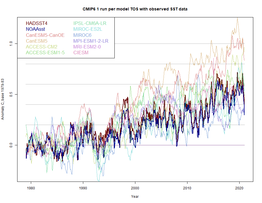
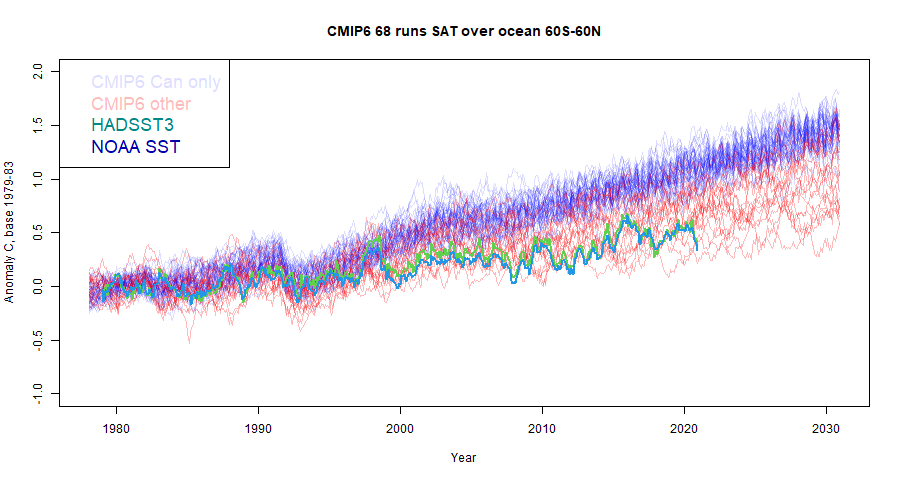
As before, the CanESM results, of which there are two, are clearly the most rapidly warming. If you exclude them, the observed is in the centre of the modelled range. For comparison, here is my previous plot in which I showed TAS with a trend adjustment from CMIP5 TAS/TOS:
Blending TOS/TAS to compare with observed land/ocean.
As said above, CMIP TAS results are often compared with modelled land/ocean, with much the same problems as in Roy Spencer's usage. Cowtan et al (2015) derived a combined TOS/TAS for CMIP5. They did a cell by cell calculation of the blend. I think it is arithmetically equivalent to use the posted land average TAS with TOS, provided the weighted combination uses the same land/sea mask to calculate areas as it did to average the temperature subsets. In this case, I used the areas that were provided with the TAS/TOS data (in the header), so I hope that is true. If not, it won't make a big difference. The land fraction was 0.287.Update 5 May 2021. I made an error in the initial post; I used the wrong column blended with sea TAS instead of land TAS. It makes a considerable difference, although the relative position of GISS is as originally described. The old plot is <a href="https://s3-us-west-1.amazonaws.com/www.moyhu.org/2021/05/blend1.png">here</a>. The zip file linked below has been updated.
I blended always TOS/TAS runs that had the same variant number, although that common value may vary from model to model. Again, I chose one blend from each model, and compared with GISS land/ocean:
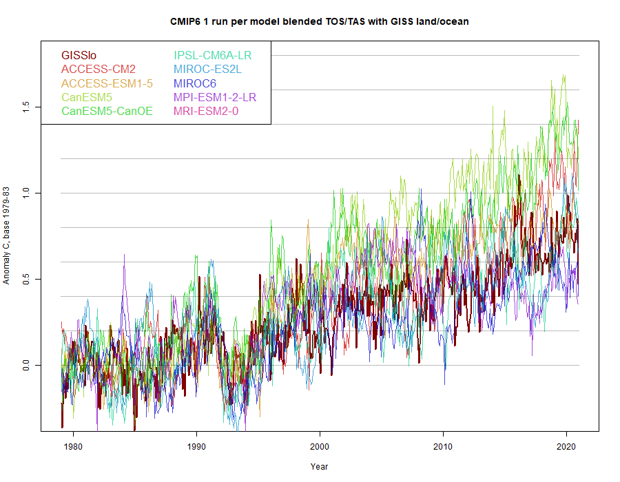
Again, the CanESM results warm fastest, and GISS sits on the warm side of the other results. For comparison, I plotted what would happen using TAS global alone, as is often done
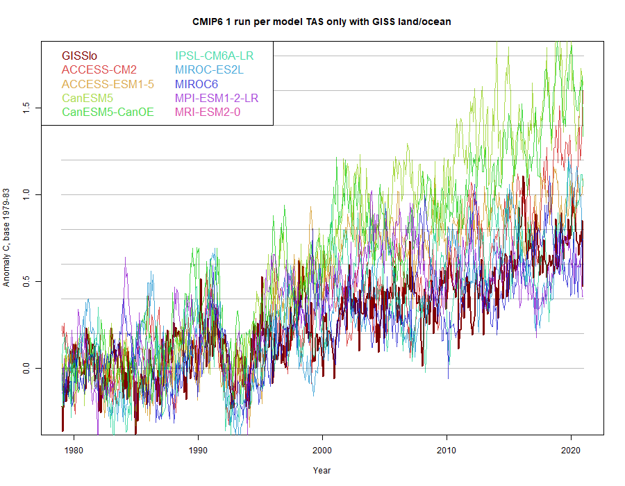
Even excluding CanESM, it now appears that modelled results run warmer than GISS. They are also a lot more variable. It is important to compare with the blend.
I blended always TOS/TAS runs that had the same variant number, although that common value may vary from model to model. Again, I chose one blend from each model, and compared with GISS land/ocean:
Again, the CanESM results warm fastest, and GISS sits on the warm side of the other results. For comparison, I plotted what would happen using TAS global alone, as is often done
Even excluding CanESM, it now appears that modelled results run warmer than GISS. They are also a lot more variable. It is important to compare with the blend.


There's a paper in this - if you're interested, drop me an e-mail (firstname.lastname at bom.gov.au) and I can put you in touch with some potential collaborators.
ReplyDeleteThanks for the post Nick. I've wanted to check this in CMIP6 and would like to do so as part of a team, get in touch if you're interested.
DeleteMy email can be found on CV at https://science.jpl.nasa.gov/people/MRichardson/
Thanks, Blair
DeleteEmail sent
And thanks Mark,
ReplyDeleteEmail is on the way
Nick,
ReplyDeleteVery nice work.
I am looking at your csv files and trying to compare the models to my temperature data . The CMIP6 data you have looks a a little bit noisy. So I calculated monthly normals from them t convert to anomalies. I get to compare them but the model data still looks noisy on a monthly basis. Are you sure the timing (month) is correct ? Of course I could well have made a mistake instead !
Thanks Clive,
DeleteThe land TAS was very noisy; combining with TOS calmed it quite a lot. I think the monthliness is correct; the greater risk is probably that I have used the wrong column of the big tableau. You might like to check some data from the UniMelb site; it is voluminous, but all in ascii, despite the .GAM suffix.
Clive,
DeleteIndeed I did make an error in blending, and the problem was the wrong column of the big tableau. I have posted a correction, and updated the stored csv file. Only the blend is affected, so I don't think it explains your observation; in fact the blend has become noisier.
For each model I tried to calculate the monthly normals temperatures between 1961 and 1990, and then subtract these to get all the model "anomalies". These can then be compared directly to the measured global temperatures on the same baseline. It is quite possible I still have a bug! However your new csv file now have 12 monthly temperature variations of up to 5 degrees, which seems very high. The old one was < 1 degree. I'll take a look at the UniMelb site. thanks !
ReplyDeleteIt looks like Scafetta recently published a CMIP6/obs comparison paper... but I saw no evidence that he recognized that there was a potential issue with blending land & ocean temperatures (I have to say, I'm not impressed with the peer reviewers for the paper... I would have expected them to catch the land/ocean blending, inappropriate comparison of UAH data to surface data, specious arguments for excluding RSS data... the list goes on). See https://judithcurry.com/2022/09/25/cmip6-gcms-versus-global-surface-temperatures-ecs-discussion/
ReplyDeleteYes, that aspect is certainly missing. I thought it was weak paper; it didn't have anything very radical to say about ECS, and seemed to go in circles (cyclomania?).
Delete