| People tend to want to argue in terms of what Hansen said about the scenarios. As I maintained earlier, that isn't the right test. Scientists work with scenarios because there are some inputs to the model that they just don't know (like how much carbon we'll burn). And there is no use parsing their language to learn more. What counts is what happened. But just to review, the usual claim is that H referred to Scen A as "Business as usual" in a Senate hearing. But that doesn't mean he thought that was what would happen. He actually said in the paper that Scen B was most "perhaps the most plausible". Hansen did muddy the waters by constantly referring to the scenarios in terms of emissions. In fact, his program used as input the actual gas concentrations, which he often describes as forcings. He does blur the two; a key discussion is on right, where he does describe the scenarios in terms of forcing. |  |
While looking up scenario numbers, I found some detailed discussion in threads from 2008 on ClimateAudit (here, here, here, and here). They were calmer times, and the discussion is often reasonable. I'll quote from Steve McIntyre's conclusion of the second post
As to how Hansen’s model is faring, I need to do some more analysis. But it looks to me like forcings are coming in below even Scenario B projections. Thus, if Hansen’s projections over-state what we’re experiencing in 2005-2010, then this does not per se invalidate Hansen’s model, as some people are too quick to conclude. To the extent that the differences lie in lower than projected forcings, I’m not prepared to place fault on the model for those defects. Whether the forcings account for the defects is a different matter and it would be interesting to run the 1988 model with actual GHG concentration changes – an experiment that’s long overdue and which would end much speculation about the merit or lack of merit of Hansen’s 1988 projections.I think rerunning code from 20 years ago (then, now near 30) is less feasible than he thought.
There are two sources for the actual gas inputs to the GCM. One I linked to (RealClimate) in the last post. It was the original data for a paper in the following year (1989), so the numbers could have been updated slightly, but should be the same. The others were files made available through Gavin at RC. Their provenance is discussed length at CA; it seems to have involved a degree of digitisation. However, the general view sems to be that despite some noted oddities, they were basically accurate. The CA link is here. I have downloaded them, and made equivalent CSV files, which I have put into a zipfile here, including the 1989 file. In the CSV files, I have reduced the absurd precision (to 5 sig).
Here are the actual numbers for 2015, from that 1989 file, with CFC nums from here:
Here are the corresponding numbers from the files sourced at CA:
Scen A  410.1  0.3426  2.336  0.814  1.333
Scen B  406.1  0.3364  2.284  0.719  1.182
Scen C  369.5  0.3364  1.929  0.366  0.618
Actual  399   0.328   1.83 0.23 0.52
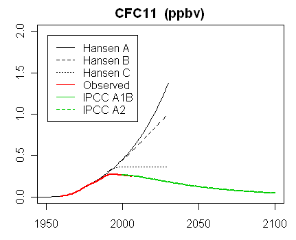
I think the first (1989) set is more reliable. Hansen said in his 1988 paper, Appendix B, that CO2 in Scenario C settled to 368 ppm, and CH4 at 1.916 which matches. So on that basis, I think it is clear that CO2 is close to Scenario B, N2O also, while CH4 and the CFC's are below Scenario C. Actually there is a wrinkle here; Hansen doubled the CFC numbers to allow for other CFC species, so on that basis they are actually well below C. That is actually a tribute to the Montreal protocol, which came after Hansen's 1988 paper.
I was going to make graphs, but I think the CA ones (from here) will do, although they are based on the econd set of figures:
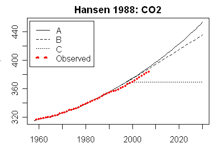 | 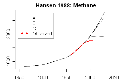 |
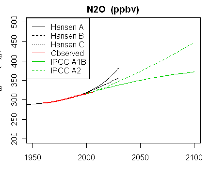 | |
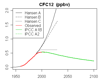 |  |
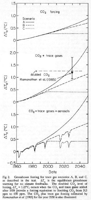
Finally, I'll include Hansen's Fig 2b, which shows the forcing effect combined with postulated volcanic eruptions in Scenarios B and C. The 1995 explosion was well matched by Pinatubo in 1991, but we're still waiting for the 2015 bang, though there have been several smaller ones.
Scenario data zipfile (txt and csv) here


Nice work. I think the spirit of the scenarios would suggest other GHGs (i.e. the 15-minor field here) should be accounted for in the CFC forcings.
ReplyDeleteThere's also a wrinkle in the Methane concentrations. Checking the start (mid-1980s) of the current Methane record at AGGI or this page against Hansen's scenarios, Hansen's numbers are offset about 100ppb higher. This might have something to do with a mid-latitude NH bias in methane observations used at the time(?), methane being a not-quite-well-mixed GHG. Offsetting Hansen's absolute numbers down by 100ppb through the record makes Scenario C at 2015 a close match to the observed concentration.
Re-running the model would indeed be very difficult, if not impossible. But you can do something very much easier, which is very nearly as good: simply re-scale the model years output to "total forcing" (which would probably be mostly the CO2; I suspect the CFCs would be too small to matter, maybe the methane is large enough to notice). That ignores thermal inertia effects (and changes in the mix of gases), but I doubt they would be terribly significant for the amount of re-scaling required. it would be an interesting exercise, at least.
ReplyDeleteI actually took a stab at this a while ago, using forcing estimates for Hansen et al.'s scenarios from here, and estimates of observed forcing up to 2011 from AR5, then rescaling by regressing each forcing series against time. Results here. The observed forcing is brought down in the early period by volcanic activity, so I also did a run excluding volcanic forcings, with pretty similar results. Either way, the rescaled model projections are a pretty good match for GISTEMP.
DeleteAs for re-running the model, it may not be quite as difficult as it seems. IIRC, the model in question is GISS Model II, which is the basis of EdGCM. Sadly, I can't afford the $200 asking price, but perhaps at some point I might try to get a comparison run done using the 30-day trial period.
Yes, I agree its nice work, Nick. I did have a question about the earlier post however. It looks like the baseline for the UAH and RSS data may be wrong as they start well above Hansen's projections in 1979. Why did you baseline these that way?
ReplyDeleteDavid,
DeleteIn my original post, I explained the offset:
"With multiple indices there is always an issue with differently calculated anomalies. Here I used the GISS Ts index unchanged; it does (still!) match Hansen's observed data in the overlap period. I then shifted the other indices so that they would have the same average as GISS Ts from 1980 to 2009 (30 years). But I've allowed users to modify this offset if they have a better idea."
So that is why; the satellite sets are flatter over the period. It is indeed arguable that they should start at the same level.
I see that the post I linked has got messed up format in Chrome; I'll investigate.
I've fixed the format problem. On looking at it, I don't think the baselining is badly unfair to the sat data. The center of the baseline period is 1994/5, not so far from 1988. I can't really do better with a 30 year baseline (OK, maybe start 1979). And I think the discrepancy at 1988 is modest.
DeleteI go by eyeballing the offsets at WfT at 1979, and try to manipulate Nick's offset to get approximately the same "look" I see on WfT. For RSS I set Nick's offset at -0.05. I have to set the offset for the series before clicking the radio button for the series. Probably makes no sense.
ReplyDeleteApologies that this was apparently reclassified as spam. Blogger rarely does this lately; I'll monitor more carefully.
Delete