The underlying principle is that in making an anomaly you should subtract your best estimate of what the value would be. That leaves the question of how good does "best" have to be; it has to be good enough to resolve the thing you are trying to deduce. If that is the change of global temperature, your estimate has to be accurate to the effect of that change.
If you add a global G to a station mean, then the mean of the result isn't right unless mean G is zero. There is freedom to set average G over an interval, but only one - not over all station intervals. So as in the standard method, you can set G to have mean zero over a period like 1961-90, and use station means over that period as the offsets. Providing there are observations there, which is the rub. But much work has been done on methods for this, which itself is evidence that the faults of naive averaging are well known.
Anyway, here I want to check just how much difference the real variation of intervals in temperature datasets makes, and whether the iterations (and TempLS) do correct it properly. I take my usual collection of GHCN V3 and ERSST data, at 9875 locations total, and the associated area-based weights, which are zero for all missing values. But then I change the data to a uniformly rising value - in fact, equal to the time in century units since the start in 1899. That implies a uniform trend of 1 C/century. Do the various methods recover that?
Update - I made a small error in trends below. I used unweighted regressions, which allowed the final months of 2015 to be entered as zeroes. I have fixed this, and put the old tables in faint gray beside. The plots were unaffected. I have not corrected the small error I noted in the comments, but now it is even smaller - a converged trend of 0.9998 instead of 1.
So I'll start with land only (GHCN) data - 7280 stations - because most of the naive averaging is done with land stations. Here is the iterative sequence:
|
|
As in the last post, the first iteration is the naive calculation, where the offsets are just the means over the record length. RMS is a normalised sqrt sum squares of residuals. As you see, the trend for that first step was about half the final value. And it does converge to 1C/Cen, as it should. This is the value TempLS would return.
I should mention that I normalised the global result at each step relative to the year 2014. Normally this can be left to the end, and would be done for a range of years. Because of the uniformity of the data, setting to a one year anomaly base is adequate. For annual data, base setting is just the addition of a constant. For monthly data, there are twelve different constants, so the anomaly base setting has the real effect of adjusting months relative to each other. It makes a small difference within each year, but if not set till the end, the convergence of the trend to 1 is not so evident, though the final result is the same.
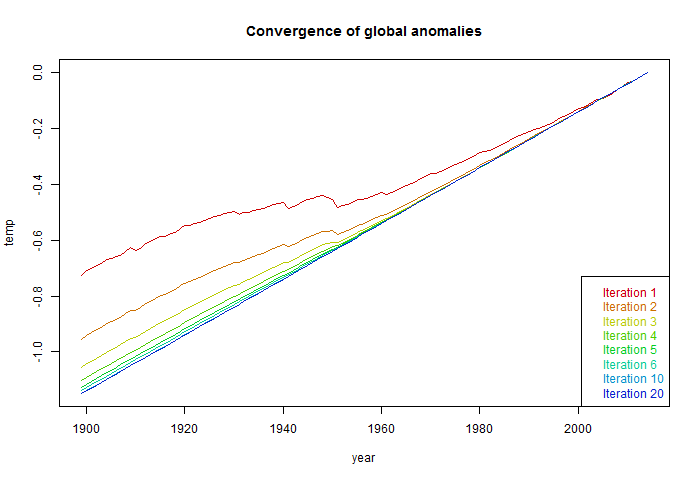
So normalised to 2014, here is the plot of the global temperatures at each iteration:

The first naive iteration deviates quite substantially, with reduced trend. The deviation is due solely to the pattern of missing values.
Now I'll do the same calculation including sea surface temperature - the normal TempLS range. The effects are subdued, because SST grid values don't generally have start and end years like met stations, even though they may have missing values.
|
|
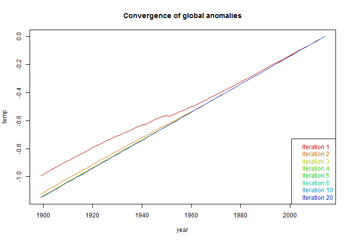
The corresponding plot of iterative G curves is:

The deviation of the first step is reduced, but still considerable. Convergence is faster.


Very nice !
ReplyDelete" I should mention that I normalised the global result at each step relative to the year 2014. Normally this can be left to the end, and would be done for a range of years"
In the real world how do you normalise TempLS? Do you calculate 12 monthly normals 1961-1990 ? If not how do you avoid doing so. NCDC and Berkeley use an earlier normalisation 1959-1980 which then causes about a 0.15C offset compared to CRU and GISS.
Thanks, Clive,
DeleteYes, I do compute 12 normals. In fact, the monthly calc is effectively 12 separate time series calcs, combined at the end. It makes a subtle difference to the effect of anomaly base. For an annual calc, shifting the base period just adds or subtracts a constant. But for monthly, it shifts the months relative to each other. So if, in 1961-90 Junes were unusually warm relative to May/July, then ever after June anomalies will tend to show as cool. The inverse pattern will be impressed. That's when having as long a base period as is practicable really helps.
To follow up, there is a third-error there that I have never corrected. If there is warming, then over 1961-90, Decembers of each cal year tend to be warmer than Januarys, because of warming trend, typically 0.01-0.02 °C. And that superimposes a sawtooth wave of that amplitude. A sawtooth wave has a very small effect on trend - of order amplitude/duration.
DeleteThat shows up here. For Land/Ocean, the trend does not converge to 1, but to 0.999637. That is because of that effect.
"third-error"
DeleteI meant third order error. But I actually made a second order error with the trends. I forgot that I had set x-values to 0 where w=0 (missing values). But when calculating trends, I used unweighted lm(), so the last months of 2015 counted as zero. This has small effect, since I was setting 2014 to zero as the anomaly base. But now the trend effect due to the mean drift over a year is just 0.99998 instead of 1.
I had assumed that the station offsets as described by Tamino had the advantage that all station data could be incuded. However, when I tried to normalise these station offsets to a fixed period 1961-1990 it didn't work.
ReplyDeleteAnom(mys) = T(mys) - (norm(m,lat,lon) - offset(ms)
Now I realise why. The problem with using any fixed period for the 12 normals is that it only applies for stations with measurements in that period. The normalisation itself is affected by these 'missing stations'. The only way round this is to exclude these stations completely or to interpolate their values into the normalisation period. However I strongly suspect that interpolation itself exaggerates any warming trends. I think Berkeley Earth suffers from this because they have to interpolate long times and distances to incude all stations. Too much smoothing reinforces underlying trends.
You either use all stations and normalise to the full period or use a fixed period and discard those stations with insufficient data.
Clive, I'm not sure what the problem is here. You minimise sum squares to get the offsets and common T. You only need to worry about the fixed period afterwards. I find Tamino's method unnecessarily complicated; if you're minimising SS, there is nothing gained by breaking into cells.
DeleteAnyway, that's how it works with TempLS, and with the iterative version that I've described. You aggregate by least squares fitting, effectively as 12 separate month analyses, each with a degree of freedom to add any number from the global to the offsets. Then you use these dofs to align with normals over a fixed period.
Nick,
DeleteYou alluded to the problem in your previous post.
"The normal remedy is to adopt a fixed interval, say 1961-90, on which G is constrained to have zero mean. Then the L's will indeed be the mean for each station for that interval, if they have one. The problem of what to do if not has been much studied. There's a discussion here. "
In fact there was not any real discussion at all in that article by Steve Mosher.
Lsm are the offsets for any station. If that station has no data withing the normalisation period then it cannot contribute to the zeroing of Gmy. As an extreme example lets take a station is at the summit of everest so it's offset is allways about 20C. The station only has data from 1850 to 1940. This means it will move Gmy to lower values for early years. There is nothing that can be done about that bias using a fixed normalistion period.
What I did instead (and I am not saying this is right) is the following.
Suppose we had perfect coverage in all grid cells. Then we can measure exactly the average temperature in each region Tmy(Lat,Lon). Insetad we have a changing population of stations any value will be biased. But by how much? Well we can estimate the 12 offsets for each station Lsm by calculating the mean difference between the measured average Tm(lat,lon) and the individual station measurements Xm, averaged over all years when the station is present.
Now we can calculate a new set of regional averaged temperatures Tcmy(lat,lon) = mean (Xms -Lsm), where the avergae only includes stations present in that particular month and year.
You can iterate round the loop replacing with the new values to recalculate Lsm. In reality the result converges after just 2 steps. This IMHO is the best estimate possible for a regional Xm(lat,lon) . Note now that the Everest station now only effects years and months in which it appears. The downside is that the normalisation of G is done using the corrected average Tmy per grid. You have to use the full time period rather than 30 years. Otherwise Everest type stations won't contribute.
Clive,
Delete"In fact there was not any real discussion at all in that article by Steve Mosher."
Well, the methods are at least described. They are RSM, FDM and CAM. The first two have various problems, and the third does abandon stations. I'm recommending a fourth method - least squares - which uses all stations. It applies at the stage of aggregation - globally is my preference, but at cell level if you must (Tamino). Once aggregated, the issue of the loose degree of freedom needs to be pinned down, but we're then dealing with aggregates, not stations.
Your cell iteration sounds something like my method. Tc_my is like G. If you alternate G=av_s(T-L) and L=av_y(T-G), that's what I'm suggesting, though I would start with G=0, you seem to start with L=0. But there is no time period issue. No period is mentioned. You use all the data. For me, of course, these are weighted averages.