Interpolation, proxies and uncertainty

I have now posted three simplified emulations of the Marcott et al reconstruction, here, here, and here. Each used what I believed to be their assumptions, and I got comparable means and CI's. And I think the Marcott assumptions are fairly orthodox in the field.

But I've been wondering about the noise structure, and in particularly the effect of the extensive interpolation used. The proxies typically have century+ resolution, and are interpolated to twenty year intervals.

The interpolated points are treated as independent random variables. They have about the same uncertainty (amplitude) as data points. But they are certainly not independent.

I find it useful to think about interpolation in association with the triangular basis (shape) functions of the finite element method. I'll talk about those, and about the kind of linear model approach to reconstruction that I described in my last post. Below the jump.

Basis (shape) functions

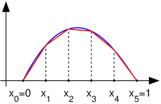
These are described  here. For this context, they are the simplest possible - triangles of unit height. From Wiki, here's a linearly interpolated function:



That has regularly spaced intervals, but that's not at all essential. The corresponding basis functions are shown here:



Wiki doesn't show this well in the diagram, but the interpolate is achieved just by multiplying each basis function by the corresponding data point and adding the results, as shown here:


A major elegance of the finite element method is that you can then switch attention to the elements (intervals) and assemble the result (interpolate) by operating on the fractions of the basis functions that lie with ine element.

Linear model

In the last two posts (here and here.) I have described how the collection of proxy data (T_tp) can be fitted to a simple linear model:
T_tp=T_t+P_p + error
where T_t is the global temperature function being sought and P_p are offsets associated with each proxy (index p). When I did that, the data points were interpolated to 20-year intervals, and that was the spacing of t. So there were 565 T_t parameters over 11300 years.

With 20-year basis functions B_t (τ) you can interpret T_t as a continuous function of time τ:
T(τ)=Σ T_t B_t (τ)
That's the linear interpolate; the T_t are still the parameters we're looking for by fitting.

In principle, I believe you should enter just one equation for each data point, which gives a reasonable chance that the residuals are independent. But how to make that equation?

Collocation

I'll now write s instead of t when thinking about the irregularly spaced data times
You could say just that a data point T_sp stands on its own, and the equation associated with it is:
T_sp=T(s)+P_p + error
T(s) would be expressed as Σ T_t B_t(s)
That looks like potentially a large sum. However, only two at most basis functions overlap s, so only two of the T coefficients are implicitly involved.

However, that would give low weighting in the equation system to proxies that had sparse data values. They may not deserve that, because the data value may be representative of a longer interval. In many cases, sparse proxies are so because it was decided that there just wasn't much point in expressing numbers at finer resolution; they just don't change enough.

Galerkin

The extreme alternative view is to say that the data point is representative of the interval up to the next point. That's really what is assumed when the data is linearly interpolated. In our terms the data point represents a contribution measured by its product with its basis function.

Well, that's OK, but we need numbers. In the Galerkin method, that is obtained by multiplying the continuum proxy equation
T_ps B_s(τ)=T(τ)+P_p
by that same basis function B_s(τ) and integrating. The integration is in principle over all time, but the basis function is only non-zero on the intervals adjacent to s.

Implementation

I'm currently trying to implement the Galerkin method. The results are noisy, and I'm not sure if I'm getting it right. I'll report.