A proper uncertainty dimple

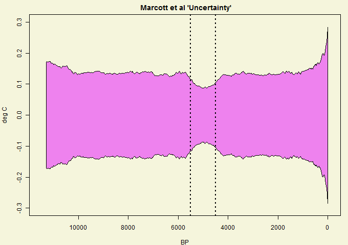
In my previous post I discussed proxy reconstructions, anomalies and uncertainties. I looked at a stochastic model for a single proxy, and derived an expression for the CI. This was (1σ):
+- sqrt(DKD^*) where D is a simple matrix which implements the mean subtraction step of anomaly formation and K is the covariance matrix of the time sequence residuals.

I have now applied this to the case of AR(1) residuals. This gives a pattern similar to the Marcott case discussed at Climate Audit. There's a bonus in that fitting the shape gives an estimate of the AR(1) lag factor.
#Update - section relating this model to recon, and R code added

I used the same general scheme as in the previous post to generate the AR(1) sequences. I set the scale to match the Marcott plot in century steps. Here is that plot from Climate Audit:


I actually used the DKD product to compute, though an analytic expression can be derived. With r=0.6 in century units, I plotted 700 proxy realizations, plus the 1σ and 2σ bounds. I've scaled so that the 2σ look like the shape of the Marcott 1σ, but doubling the scale would match the 1σ shapes. Here's the plot:



The scale is reversed, but it is symmetric. I think both the shape and depth of the dip match fairly well for r=0.6.


Update - fun fact.
The dimple has an analytic form for AR(1), parameter r, at least if the base region has an odd number of points M. It is:
Let m=(M-1)/2, i be the time index centered at the middle of the base
Let y0=(1+r)*(1-2*r/(1-r^2)*r9/M)
If i≤m (i in base): k_i=r^|i-m}-r^|m+i+1|
If i>m:  k_i=1+r-r^(m+i)-r^(m-i)
Then variance y_i=1+(y0-2*k)/M/(1-r)

The function is like a cosh in the base, then asymptotes exponential to the far field.

Noise model and proxy reconstruction

In this post, I've stripped the mathematics down to just a noise model AR(1). I should review how that relates to a proxy reconstruction.

I've drawn 700 realizations of that noise in the plot. You could think of a toy recon in which 700 proxies around the world, some hot, some cold have a fixed base temperature, with one of those noise realisations added.

So we'll make a reconstruction from these. We take anomnalies (using D). This strips out the varying fixed base temperatures, and leaves 700 realisations of anomalised noise, which will each have the CI's shown here.

Then we average them. That will be the recon. The CI's are scaled down by sqrt(700), leading to this plot:

Code

#Code written to calculate for CIs of an anomaly calculation, AR(1) noise
#Nick Stokes www.moyhu.blogspot.com 13/4/13

# Set up covariance matrix K for AR(1)
r=0.6 # AR(1) parameter
X=113 # timesteps
x=1:X-1 # timescale
K=r^(abs(outer(-x,x,"+")))
# Set up anomaly op
base=45:55+1; M=length(base);
D=K*0; D[,base]=1/M; D=diag(X)-D;
# Matrix products to get variance
E=D%*%(K%*%t(D))
ci=sqrt(diag(E)) # variances
#Analysis complete
# Now plot sigma and 2*sigma CI's
x=x*100 # rescale to years
png("dimple.png",width=1000, height=500)
plot(x,ci,xlim=c(0,X*100),ylim=c(-4,4),type="n",xlab="Years BP")
# Now make proxies for plotting
cl=rainbow(22)
h=range(base-1.5)*100
rect(h[1],-4,h[2],4)
for(i in 1:100){
u=as.vector(arima.sim(n=X,list(order=c(1,0,0),ar=r),sd=sqrt(1-r^2)))
lines(x,u-mean(u[base]),col=cl[i%%22+1]) # proxy curves
}
for(i in -2:2)lines(x,i*ci,lwd=(i!=0)+1) # CI curves
dev.off()