Below is the graph (lat/lon) of temperature distribution for September. There is also an interactive world map.
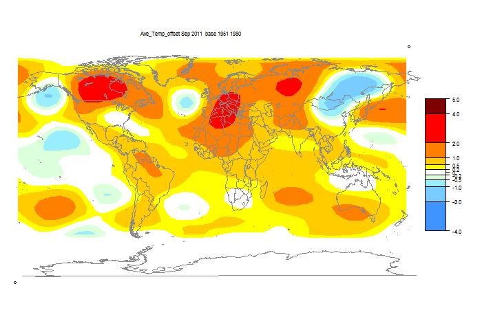
This is done with the GISS colors and temperature intervals, and I'll post a comparison when GISS comes out.
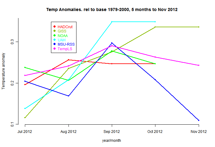
And here, from the data page, is the plot of the last four months:
Finally, here is the interactive worldview of Sept surface temperatures. Just click on the yellow squares to see different views of the Earth. The bottom square is the S pole view. The first click takes a second or two for loading.


Maybe you've answered this before but what's with the swirling at the North Pole in the Arctic?
ReplyDeleteNo, no-one has asked. It's an interesting artefact. The way I do the equal area cells is to divide each latitude band into the right number of segments. The pole doesn't fit that system, and the cells there work out triangular.
ReplyDeleteThat doesn't quite answer the question - the effect doesn't seem to happen at the South Pole. And because it is smooth, it must involve the spherical harmonics somehow. And deriving their coefficients doesn't involve the cells.
I've been meaning to look into it more - you've encouraged me.
Robert,
ReplyDeleteI should thank you for prodding me to look at that spiral effect. It was a plotting bug - minor in its effect, but of some significance. It only affected the globe plots, not the flat one. And it was only noticeable at the N Pole.
Here's how it happened. I create a virtual globe in which 0.4 deg squares are colored by their spherical harmonic values. That is 257828 squares. They are ordered in latitude bands, starting at the S pole and ending at the N.
There is a large intermediate calc, and to fit this into memory I do batches of 10000. But I made a counting error of 1 with each batch, and There were 25. It accumulated and so by the N Pole, they are 25 squares out. At the equator, tthe error is half, so it is about 5° of longitude at the equator, but of course much more at the N Pole. It's not noticeable much below the pole, because it is virtually the same, lat band to lat band. But at the pole it has that nifty spiral effect.
Which has gone - I fixed the bug. It's still there back in the July plot.
Nick,
ReplyDeleteI forget, does your global anomaly calculation use interpolation?
Also, at some point you were going to integrate ghcn3 and hadsst3. I'm curious to see what the new data sources and interpolation does to the various "controversial" time periods, ie 1910, 1940s, 1998+.
Finally, according to their web page, the Berkeley group will be releasing their code and data by the end of the month. Interesting times ahead (presumably more condemnation of Muller for not giving the "expected" result).
CCE
ReplyDeleteThanks for the info about Berkeley. Well, things needed livening.
The global anomaly uses least squares, so no explicit interpolation. However, whenever you average a sampled quantity, there's always some requirement that they are representative.
I'm not using HADSST3 at the moment, because it does not have current months (AFAIK). But yes, a study of what difference HADSST3 makes with GHCNV3 is overdue. I have never found that GHCNv3 is much different to v2, but SST3 does make a difference.