Ver 2 - Regional spatial variation.

The last thing I wanted to get working in TempLS before posting was mapping regional spatial variation. But that's been more difficult than I expected. It comes hard up against resolution and the irregular distribution of stations. But these turn up in somewhat unexpected ways. It's been instructive, so I thought I could blog about that while I'm thinking about what to do next.

My idea was to look at roughly rectangular regions in a similar way to the example of the globe with spherical harmonics. A more appropriate family of functions there are trig functions - a standard Fourier series in 2D, although fitted by least squares.

I looked at ConUS, where NOAA has plots that I can compare with. The results were not disastrous, but not very good. The basic reason is that the number of US stations in ConUS (especially currently) is much smaller than the number NOAA would use.

I could use a larger set, eg USHCN. But I'm looking for a general purpose tool based on GHCN that will work for other places that don't have this alternative. I'll describe progress below the jump.

Orthogonal Functions

First a digression on orthogonal functions - why we like them, and what if we can't get them. As I've said in previous posts, LS spatial representation comes down to saying that the temp or trend is a linear combination of some smooth functions (maybe a hundred or two). After eliminating the variables associated with local station properties, a symmetric matrix equation results

S*p=r

where p are the parameters or coefficients.

Orthogonal functions are chosen to try to ensure that S is well-conditioned. That means that there isn't a large range of eigenvalues. Put another way, there aren't eigenvalues that are very small, which would make the matrix close to singular.

Small eigenvalues hurt, because they represent combinations of approximating functions that can be added with little effect on the result. In our context, without much affecting the sum of squares. But they affect the appearance of the solution. The result is the solution isn't uniquely defined. You can try to compare two outcomes and get what looks like different results. But, even worse, the differences can't be said to have physical significance.

Orthogonal functions like spherical harmonics are actually orthogonal with respect to integration over the region. We don't have that - there are sums representing results at an irregular set of measuring points (the stations). One can hope that these would approximate the effect of integration, but this will fail when the functions have enough variation that they change a lot between stations. That's the resolution issue. What I've been finding is that this happens earlier than I had expected. I think this relates to the irregular distribution.

ConUS

I took an an example problem the task of plotting temperature anomalies for the lower 48 states for 2008. Here's NOAA's version of this result:
.

Using TempLS' mask facility, I chose stations by the US country code, 425, with some lat/lon restrictions to exclude Alaska and Hawaii:

"ConUS" = tv$country == 425 & tv$lat<51 & tv$lon > -130 & endyr > 2007,

Then I defined the minimal lat/lon "rectangle" containing these stations. The Fourier approximants were trig functions periodic on this rectangle, down to a certain minimum wavelength. I used a parameter N which approximately expressed the maximum number of wave periods allowed. I say approximately, because there were more in the horizontal than the vertical.

I originally allowed all ConUS stations, which gave reasonable numbers (1841). But then I added the restriction to stations posting results in 2008, which brought the number of stations down to 122. That's still fine for a countrywide average, but not much for resolving spatial variation.

Low resolution

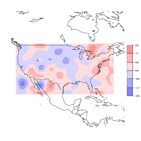
I started with N=2 - trig functions which at their highest frequency only have about 2 periods across the country. The result looked like this:


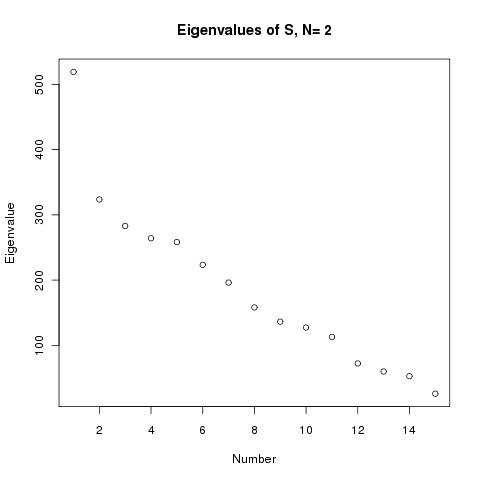
No detail, although it broadly gets the warm and cold parts right. There were 15 approximating functions. On a Fourier basis, you'd expect the eigenvalues of S to drop by a factor of 4 as the frequency rises, but a plot actually shows:

The drop is by a factor of 20 - not enough for major artefacts, but a problem looming.

More resolution

So try N=4. Now 35 approximating functions. The eigenvalue plot now looks like this:


The minimum eigenvalue is now 1.4, down by a factor of about 400. So there may be problems. Here's the plot:

It actually looks better within the country. Same effects but better resolution. But there is a suspicious blob in the Bermuda triangle, and over Canada.

Is this a problem? The likely reason we see trouble there is that, of course, there are no stations used there. The Bahamas blob affects Florida a little, but not much.

One remedy might be to include offshore stations too, including ocean. That would probably do better, but isn't in line with the original aim, which was to get just US results.

Still more resolution

Move on to N=8. Now we have 91 approximating functions. The eigenvalue plot looks like this:

Now the eigenvalues get down to order 10E-5, from a max of 622. That's definitely problem territory, and there are about 20 in that region. Here's the plot:

It's really gone haywire.

PCA

We can try a principle components type remedy. R makes it easy to just get the matrix of eigenvalues corresponding to a larger subset of eigenvalues, and that gives a subset of approximating functions with better orthogonality. Trying that with N=8, allowing a 100:1 range, we're down to 68 functions, and the plot becomes:

So it's at least back within range, and in fact broadly gets the pattern right. It's arguably better than the N=4 result. With a more severe 20:1 eigenvalue restriction, we're down to 59 functions, and the result is:

Similar pattern, but with smaller variations, as you expect with reduced resolution, but may reflect removal of artefacts too.

Beyond the borders

I tried the idea of using all the stations in a rectangular block that included ConUS. The mask was
 "US" = tv$lat<49 & tv$lat>25 & tv$lon< -66 & tv$lon >-125 & tv$endyr>2007,
There are now 171 stations, up from 122. We still have N=8, with 91 approximating functions. There was some good news with the eigenvalue plot:

They taper down to a minimum of 0.7, about 1000 times down from the max, but it's a lot better. Restricting to the 100:1 range only cuts out 6 stations functions, and gives this plot.

Some rather odd spots below Calif, but otherwise reasonable, and the US comparison is probably the best we have seen.

Conclusions and thoughts

To emphasise again, we're trying to get a picture of an area like ConUS with only 122 stations in 2008. With USHCN we could have many more and could do much better. But that idea would not extend to ROW.

The limited resolution plots are of some value, especially if you ignore patterns outside the region with stations.

Ver 2 may push for use of "rectangular" subregions, rather than country-shape regions, to avoid misinterpretation of artefacts. I would probably make a PCA type restriction to a 100:1 eigenvalue range the default.

A more radical idea, which I'll explore, is to move away from smooth approximators like trig functions, which get their orthogonality from phase relations, toward finite element type shape functions. These are approximately orthogonal because most of them just don't overlap, which may be more robust toward station distribution. The resulting plots would be more grid-like.