Version 1.2 of GHCN processor

I have put up version 2. It has some extra capabilities, and some improvements in layout. Like V1.1, it is eparated into a preprocessor and a main processor. You should only need to run the preprocessor once, unless a new v2.mean comnes along (or a new code version, as here).



I think users will find this version more convenient and powerful in selecting categories. You can control the year intervals for plotting and trend calculation (separately). The preprocessor now passes a file statyrdata.txt which gives the start and end of each station record, and the length (total years).

The code is here and at the document store.

Update. Carrick pointed out a bug a while ago, which I found frustrating, because I couldn't reproduce it. It turns out that it was due to bad treatment of the end year, and I couldn't see it because I was using a Jan version of v2.mean which didn't have 2010 data. Anyway, it's fixed now (thanks, Mosh) - so I'll update with v1.2.1 files. 

A summary of this series of posts is here.

User variables

 At the top of the file you will see this section:

#### Parameter definitions - these vars are ones that you might want to change

# Input file locations - change to path where yours are kept

input1 = "v2mean.txt";     # Made by preprocessor - should be in current dir
     
input3="statyrdata.txt";   # Made by preprocessor - should be in current dir 
   
input2 = "v2.temperature.inv";



# subset selection - title names appear in graph and text output - you need to write a matching condition below

title = c("Global","NH","SH","ConUS","Airport","Rural","Urban","Cut","Kept","BC","Africa");

choices = c(1,4,8,9,10,11); # select items from "title" for this run;



# plot selection;

yr0 = 1880;  # Start of the analysis period - don`t ask for trends or plots before this date;

yr1=2009; plotyrs = matrix( c(1900,yr1, 1978,yr1),nrow=2) #list year pairs, as many plots as you want;



# trend selection start and finish;

trendyrs = matrix( c(1900,yr1, 1978,yr1),nrow=2) #list year pairs, as many trends as you want;

This collects in one place the variables you are most likely to want to change.

Trend and plot years selection

Here you just list in the form c(1900,yr1, 1978,yr1) the pairs of years that you want plots and trends. This refers to trends calculations reported on the output file. Trends will be calculated for plots too, but determined by the plot years.

The format of the list is start,end,start,end... It's up to you to ensure that there are matching ends. The use of yr1 is optional, but may help when 2011 rolls around. You can have as many pairs as you like (but be reasonable).

Station subset selection

There are three steps:

1. Decide on a set of names

2. Program a set of criteria. This is the harder part. Down in the code, you'l find a list like this:

if(tc == "NH") i01 = i01[tv$lat>0];

  if(tc == "SH") i01 = i01[tv$lat<0];

  if(tc == "ConUS") i01 = i01[tv$country == 425 & tv$lat<51 & tv$lon > -130];

  if(tc == "Airport") i01 = i01[tv$airpt == "A"];

  if(tc == "Rural") i01 = i01[tv$urban == "A"];

  if(tc == "Urban") i01 = i01[tv$urban != "A"];

  if(tc == "Cut") i01 = i01[tv$endyr<1992 & tv$length>50];

  if(tc == "Kept") i01 = i01[tv$endyr>2005 & tv$length>50];

  if(tc == "Africa") i01 = i01[tv$country <190];

  if(tc == "BC") i01 = grep(",BC",tv$name)


 
The key task is deciding on the logical expression. It helps to have some knowledge of the v2.temperature.in file. The list of attributes of the object tv, taken from this file, is:

colnames=c("country","wmo","mod","name","lat", "lon","alt","ialt","pop","ipop", "topo","startyr","endyr","length","airpt", "town", "veg","urban");


I've used three of the more obscure locations to put the startyr, endyr, length information. You can use any of this info to create subsets. For example, I've used the year info for Cut and Kept - to try to separate the stations "dropped" in the early 90's. It would be best to run these with appropriate year selection.



You can see how R extends the possibilities with the "BC" example. The .inv file follows Canadian and US sites with the province/state abbreviation. So you can search with grep, and do just those entities. You could combine then if you like c(grep(..), grep(..))

Update - OK, it was late, and I forgot 3). Which is the decision for any run on what subsets to use.  That's the declaration of choices, as a list of numbers.

Results

Well, it's late tonight, and I wanted to post the code to solve some current problems. I'll post some result plots tomorrow.

Tips on File Download

I see there have been some problems in getting files down and running, so here are some suggestions that may help.





Text version of download

To download direct from the repository page, the best way may be cut and paste - other ways may lead to HTML issues. But best may be to use the document repository. I'd suggest just downloading the All-R.zip - it's very small. The zipfile has a directory structure that collects files related to blog posts. If you download All-Files.zip you'll get the same directory structure, but with results and anything else that seemed relevant.




Input files for R

Here I haven't been systematic enough. Most R files call input files with a scan() or a read.fwf(). I've sometimes referenced the files with aspects of my directory structure, whereas of course they should reflect your structure.

I'll try to make sure to reference the input files as if in the current directory. But I'll also put at the start of the program a set of commands saying

loc="path/file"

These will list the input files. You should insert your own paths and filenames (if different)

Update I'll extend this idea to putting a section near the top where all the variables (including input files) )that you might want to change are initialised. Instead of loc=, for input files I'll write "input1 = " etc

Text conventions for repository

I have tried to separate R code from my text with font changes (italic). But I'll try to improve by marking the beginning and end with comment lines
########  Start of prog.R   ###########

########  End of prog.R   ###########

The name is just a suggestion 0 if you down load from there you'll have to supply a name, which can be anything you like. But it probably corresponds to the name in the doc drop.


Readme

I'll try to put readme files in the doc repository and the zip files. These should describe where the files belong.


General

The blog post should tell you where to find the input files needed. GHCN files for example come from http://www1.ncdc.noaa.gov/pub/data/ghcn/v2/

Rememner to uncompress files before passing to R.

Other

I've heard of trouble in lodging comments. The settings, as I understand them, should provide no restrictions. Let me know if you can't get through.

Blogspot makes pesky issues for commenting without identity. You won't be able to paste, for example. But if you use any identity (Google, Typekey, Wordpress etc) it's much better. This may also help if comments aren't being accepted.

If all else fails
My email name is anstokes, and you can find me at westnet + com + au

More GHCN results.

I've put up version v1.1 of my least squares GHCN code. It now makes it possible to easily analyse subsets using any of the information on the inventory file. I've used it to calculate a number of much discussed examples. The code now runs very fast. On my fairly old PC, the biggest case (global) takes less than 100 secs. So although each special case is calculated pretty much from scratch, there's not much penalty there. The code is here, and also on the document repository.

New code features.

The program has now been split into two. The first is a preprocessor which reads v2.mean, does the merging of duplicates, and prints a condensed file called v2mean.txt. Unlike ver 1, it doesn't require prior editing of v2.mean. The idea is that once you have merged the duplicates, you don't need to do it again un til you want to deal with a new version of v2.mean.

The second part is somewhat like V1, but much more clearly laid out. It's even shorter (with the preprocessing gone) - about 170 lines. There's a lot of infrastructure with printed tables, plots with trends etc.

The selection process works thus. The 18 parameters from the .inv file have been given names, like tv.$country, listed in colnames. You declare a list of names that you'll want to use and have appear on graphs etc: 
title = c("Globe","NH","SH","ConUS","Airport","Rural","Urban"); 
choices = 1:7 #c(4,5,6,7);

In the second line, you declare the ones you want to run.
The logic of the choices is expressed in the list:

if (tc == "NH")   i01 = i01[cellnums>1296]; 

if (tc == "SH")   i01 = i01[cellnums<1297]; 

if (tc == "Airport")  i01 = i01[tv$airpt == "A"]; 

if (tc == "Rural")   i01 = i01[tv$urban == "A"]; 

if (tc == "Urban")   i01 = i01[tv$urban != "A"]; 

That's my current list, but you can change it.

Some results

Firstly, a table of trends, in deg C/decade.

Trends	Globe....	NH........	SH.........	Airport..	Rural...	Urban
No. Stations..	7280	6056	1224	2390	2712	4568
1900-2009	0.0760	0.0824	0.0690	0.0596	0.0606	0.0752
1978-2009	0.2717	0.3144	0.1106	0.2628	0.2561	0.2631

No real surprises. The main outlier is the SH, but remember, this is land stations only. The classifications of airport, rural and urban make little difference. The urban/rural differentiation is by night lighting, and I've included small towns with urban.

Remember that this is based on raw GHCN data, with no corrections made by me.

Update - there was a bug in V 1.1, which had a minor effect on the results, but which could cause a crash. It didn't affect global calcs - only subregions. Here are the recomputed trends:

Trends	Globe	NH	SH	Airport	Rural	Urban
No. Stations	7280	6056	1224	2390	2712	4568
1900-2009	0.0760	0.0833	0.0479	0.0661	0.0678	0.0761
1978-2009	0.2717	0.3297	0.1199	0.2438	0.2599	0.2721

I'll fix the posted code in all locations, calling it v1.11, and the results file.

I've posted the results file on the document repository.

Some plots

NH 1900-2009	SH 1900-2009
NH 1978-2009	SH 1978-2009
Rural 1900-2009	Urban 1900-2009
Rural 1978-2009	Urban 1978-2009
Airport 1900	Airport 1978

Comparison of GHCN results

I promised some comparison plots from the code reported in the last post, but Zeke has made the task much easier. He posted a spreadsheet with all the data nicely arranged, and I added my own data - you can find the spreadsheet "Temp Comps_NS.xls" in the drop.io repository.

Below are some of the plots and discussion.

A summary of this series of posts is here.

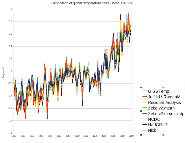
Here is the global data from 1880 ( or 1881 in my case). Details of the sources are on Zeke's post. All data is set to zero average in 1961-90.

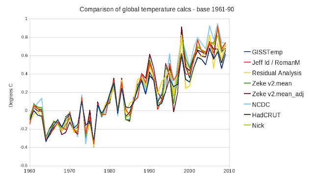
And here is a close-up of the period 1960-2009.

The agreement is good. This is encouraging, because the principle of the least squares method is very different, and bypasses all the merging of stations issues. Of course, the agreement of all the other reconstructions is also impressive.

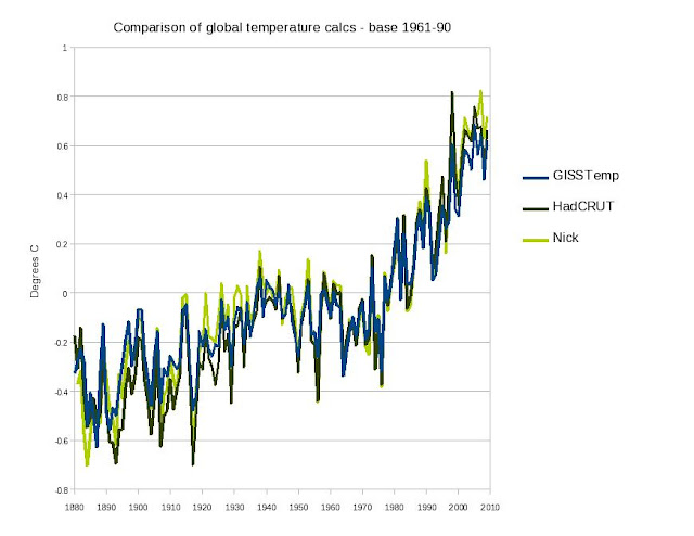
Here is a plot with just the main indices GISS and Hadcrut:

GHCN processing algorithm

As Zeke says, it seems to be a custom now for bloggers to post codes to grid GHCN data and calculate trends. Here's my offering. It's influenced by Jeff Id's program, and particularly by Romanm's Least Squares. In fact, it's an extension of Roman's offset method to the whole global set. It's fairly different to the conventional approach. It doesn't actually do gridding, or (per Roman) calculate anomalies. It's probably the shortest of the codes, and runs quite fast.

A summary of this series of posts is here.

The linear model

I'll attach a pdf file explaining the mathematics in more detail (soon). But here's a sketch. The monthly data, from v2.mean after averaging over duplicates, is in a big array x(S,m,y). The indices are station, month and year.

The model is that x can be represented in terms of a global temperature G(y) depending on year alone (not month or station) plus a local offset L(S,m) for each station S, with a seasonal component dependent on month m (but not year), plus error:
x(S,m,y) = G(y) + L(S,m) + eps(S,m,y)
I do a least squares weighted fit.

The weight function w(S,m,y) is inversely proportional to area density of stations, and of course, zero for (S,m,y) combinations where there is no data. So we're minimising (Latex-like notation) Sum_{S,m,y} w(S,m,y)*(x(S,m,y) - G(y) - L(S,m))^2

Weighting

The weight function uses a grid. But it just counts stations in each cell - no explicit grid averaging is done. The count is for each month (and year). The cell area is divded by this count to give wt(S,m,y). A conventional 5 deg x 5 lat/lon cell is used.

The design matrix system

Minimising LS gives the system
L(S,m)*Sum_{y} w(S,m,y) + Sum_{y} {w(S,m,y)*G(y)}
            = Sum_{y} {w(S,m,y)*x(S,m,y)}

Sum_{S,m} {w(S,m,y)*L(S,m)} + G(y)*Sum_{S,m} w(S,m,y)
           = Sum_{S,m} {w(S,m,y)*x(S,m,y)}

Regarding (S,m) as a single index, this is actually a symmetric system:
A1*L +B*G = R1
t(B)*L +A2*G = R2

A1 is the very big block, but is a diagonal matrix. t(B) is the transpose of B. A2 is diagonal too.

Solving

This can no doubt be solved (for local L and global temp G) using R's lm() type functions. Numerically, it is essential to take advantage of A1 being diagonal. I don't know how R can do that, and would appreciate advice.

I constructed a home-made block solver which was quite fast and apparently effective (although I have an idea for a faster version). A wrinkle is that the matrix is singular, because you coould add any constant to the global temp G and subtract it from L. So I added an equation to fix the initial G to zero.

Testing

To test the code, I created a synthetic data file with the v2,mean format, but made up of just a trend with a sinusoidal temperature (same for all stations), with a random scattering of missing data. It should give an exact answer, and it did. The test code is included here.

Results

I haven't tried hemispheres, yet, just global. I'll show in a following post comparisons with HADCRUT etc. For the moment, I just looked at global temps and trends from 1900 to present, and 1978 to present. I was particularly interested to compare with Jeff's value of 0.2476 C/dec. Here's my fig, with the result 0.2542 C.dec. (The AR1 correction is coming).

For 1900-2009, my slope is 0.0747 C/dec - well within Zeke's range.

Code and next steps

The code, and the test code, is in the repository. In a future post, I'll show results for the local seasonal temperatures from the LS fit - they are pretty interesting too.

On Polynomial Cointegration and the death of AGW

Well, I never thought I'd write a post with such a title. And I must confess that until about two weeks ago, these terms were very foreign to me. But recently, a paper by the econometricians Beenstock and Reingewertz has been circulating among sceptic blogs. It seems unpublished, but with the file called "Nature_Paper091209.pdf" there has been some jumping to conclusions. There was a brief discussion at WUWT, and more recently, David Stockwell has run a series on the topic.
  
Update.  Bart has commented has commented and linked an interesting discussion on his blog. Tamino has taken this up with a very thorough discussion (with sequels). The first properly sceptical discussion of the Beenstock paper was by Eli Rabett. 

Further update. VS has noted that the much more significant thread on Bart's blog (now much discussed in itself) is here.

Ringing phrases like:
"Therefore, greenhouse gas forcings, global temperature and solar irradiance are not polynomially cointegrated, and AGW is refuted."
ensure that those who like that sort of thing will keep it going for a while, so I thought I should try to figure it out. I'm still not an expert, but I hope what I did figure out might help.

Time series and unit roots

The theory is derived from the abstract notion of modelling a stochastic time series by a recurrence relation:
y_t + c1*y_{t-1} + ... + cn*y_{t-n} = ε_t
where ε_t is a stationary stochastic variable with zero mean (serially uncorrelated, constant variance).

This can be re-expressed symbolically using the backward difference operator
Dy_t = y_t-y_{t-1}
(a0 + a1*D + a2*D^2 +...+ D^n) y_t = ε_t
This is just binomial algebra

This is the undriven form, but a non-stochastic driver could be introduced. The corresponding non-stochastic recurrence relation (with ε_t=0) has n power solutions of the form b^t (t=0,1,2,...), and the b's are solutions of a characteristic n-th order polynomial. It is expected that these will all have magnitude not greater than 1, otherwise the process would have blown up.

The case where one or more roots are equal to 1 is called the unit root. It's important because the behaviour is qualitatively different. Instead of disturbances decaying with time, the process can just wander. It is a random walk.

Testing for unit roots

The point of the second difference form is that there is a clear criterion for unit roots. There is one root if a0=0, and the series is called I(1). There is a repeated root if a0=0 and a1=0, and the series is called I(2).

Now although people who like this sort of thing like to talk of asymptotic behaviour, there is usually no known underlying mechanics to justify this. There is just a finite period of observations. So the coefficients are never completely known (or of course, even whether it is an exact model). You can't get true asymptotics from a finite observation period.

So you can never say that a0=0. All you might be able to say is that a0 is bounded away from zero - significantly different at some level of confidence, say 95%. That's a test, and variants include the Dickey-Fuller test, and the augmented ADF test.

So when you say a series is I(1), you are saying that a test failed to yield significance. You weren't able to show, at 95% confidence, that a0 was different from 0. That's a negative conclusion, and certainly doesn't mean that you're 95% confident that the series is I(1). You're not 95% confident of anything.

In fact it's hard to quantify confidence in I(1) status in any way. Higher levels, eg I(2), likewise say that we weren't able to show that both a0 and a1 are significantly different from zero. Two failures is even harder to express as a confidence level.

Cointegration

This is used in causal arguments as follows. If, say, a temperature rise is believed to be caused by a CO2 rise, then there is a consistency requirement for the series. The long-term qualitative difference between a series with roots less than unity, and one with unit roots is great. So it would be odd to find that if temperature is I(1), so its a0 = 0 but a1 is not 0, while for CO2 (with coefs b0, b1 etc) b0 = b1 = 0. For that would mean that the temperature differences were stable, with disturbances decaying, even though the corresponding differences of CO2 could drift. That's the supposed significance of the failure of "polynomal cointegration". Though its still a big jump to say "AGW is refuted".

For let me say again, we can never be totally confident, on finite data, of statements about I(1), I(2) etc. But we don't seem to be able to quantify our uncertainty. Even less can we quantify compound statements like T is I(1), CO2 I(2), therefore incompatible.

Back to Beenstock

So how do B&R quantify their claim that AGW is refuted? Explicitly, not at all. I didn't see any confidence level attached to it. They did describe a number of tests on the CO2 series. That is, they quantified the extent to which they can say that the test for non-zero b0 and b1 failed. But oddly, there seemed to be no test statistics at all on temperature. They just said that it is I(1), apparently relying on papers by Kaufmann and others. But no confidence level was cited.

So with no quantitative confidence in one of the parts of a compound proposition, with what confidence can they say that "AGW is refuted".

They go on to make even more remarkable claims
Although we reject AGW, we find that greenhouse gas forcings have a temporary effect on global temperature. Because the greenhouse effect is temporary rather than permanent, predictions of significant global warming in the 21st century by IPCC are not supported by the data.
Again, with no physics but just a century or so of observations, they are able to say what is temporary and what is permanent.

A blatant fiddle in the D'Aleo/Watts SPPI report.

The D'Aleo/Watts report has come under justified criticism for it's silly claims about marching thermometers etc, amplified into claims about malfeasance by various scientific groups.

But there's one little thing that particularly bugs me, because I have pointed it out more than once, but it makes no difference. They say  

"See the huge dropout of data in Africa, Canada and Siberia in the two maps from NASA GISS with 250 km smoothing from 1978 to 2008"

and show these pictures:

Well, yes, quite a reduction in going from 1978 to 2008. But actually, if you go to the GISS site and ask for April 2008, what you see is not nearly as sparse.

So what is going on?

I managed to track down where the SPPI image came from. Bob Tisdale has a version of it in a post dated May 20 2008. It's an early version (current when he posted it), made with an early batch of data that came in for that month. And it's compared with the full version of April 1978.

It's a bit like that Langoliers post. But it just keeps turning up.