More on climate feedback

Recently I posted on Climate feedbacks and circuits. It was in the context of a series of articles by Lord Monckton at WUWT. The articles have continued, with more promised. Willis has joined in, though they are not always on the same page. And I've been commenting there.

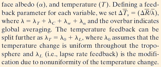
My last post was in response to much talk of positive fedbacks and instability. I showed an active circuit (borrowed from Bernie Hutchins) which wass table and would emulate the usual equation of feedback in the conetxt of climate sensitivity:
ΔT_eq = ΔF/( 1/λ₀ – Σc_i)
My main observation is that this is just like Ohm's Law, with the feedback coefficients c as conductances in parallel. The need to resort to active feedback comes from the fact that some c's, corresponding to positive feedback, may be negative. But the basic simplifying idea off adding conductances still applies.

In a much-cited review paper, Roe 2009, roe argues that feedbacks should be seen as Taylor series in disguise. I think he could have said just chain rule, since he uses only first order. But I want to develop this, because it is the basis for the method used in an also much-cited (including AR4) paper by Soden and Held, 2006. Lord M's latest post is based on the claim that S&H have made an error, but he really has no idea of what they did. So I'll try to say something about that here.

We're thinking about equilibrium climate sensitivity
S = ΔT_S/ ΔF
ΔT_S is a sustained change in global average surface temperature caused by change of forcing ΔF. But if the change in T changes other quantities x_i with i over some range, and these x generate new changes in F, e may need to take this into account. The chain rule expression says
dF = ∂F/∂x_i ∂x_i/∂T_S dT_S
Note that although we are looking for dependence of T on F, we expand the denominator F in the ratio.

The quantities x are those that contribute to F through some radiative relation that is either known or can be worked out by some atmospheric model. There is no great delay here so the calculation is quick. But x are also observable over time, probably in a GCM, so the second factors can be got by observation over time. This was the basis of the S&H method. They looked at a number of GCM implementations of the SRES A1B scenario over a century. In this, GHGs rose for a period of some decades, but then rose no further, giving a reasonable version of equilibrium change.

The variables S&H looked at were temperature T, water vapor, and surface albedo. They list various reasons why the approach is not suitable for cloud feedback, and so deduced that as the remainder, since the feedbacks add to inverse sensitivity. This emphasises that the method is for breaking down; you can't get ECS from the components.

The interesting one here is T. It expresses the Planck feedback idea of the previous post, that higher T radiates more energy, lowering (or balancing) F. But what T to use? Lord M could not be shaken in his belief that S&H used the temperature of the "emission layer", about 255K, even though there is not the slightest mention of that in the paper. In fact, it isn't good to use any global average T, since IR emission responds to the local and immediate T, and in a non-linear way.

So S&H broke T into a whole lot of local variables, based on the GDDL GCM grid, depending on time of day and year, latitude and altitude. Here is their description:

To compute Kx, we first calculate the control top-of-the-atmosphere (TOA) radiative fluxes using 3-hourly values of temperature, water vapor, cloud properties, and surface albedo from a control simulation of the GFDL GCM. For each level k, the temperature is increased by 1 K and the resulting change in TOA fluxes determines (∂R/∂T_k).

It doesn't say how long, but I presume for a year. That gives the necessary ∂F/∂x_i. Then they get the rate of change thus:

The model response for each variable x is computed by differencing the projected climate of years (2000–10) from that of (2100–10); (dx/dT_s) = (x^(2100-2110) - x^(2000-2010))/(T_s^(2100-2110) - T_s^(2000-2010)). The response is then scaled by the appropriate radiative adjoint (K_X = (‫∂‬R/‫∂‬x)) to yield the climate feedback parameter for that variable, λ_X = K_X(dx/dTs),

The products are formed for each cell/time and then average for total ∂F/∂T ∂T/∂T_S to get λ_T. They then break this down further into what they call Planck feedback λ₀, which expresses the effect of chaging T uniformly, and a lapse rate feedback λ₀, which expresses the effect of differential T change:



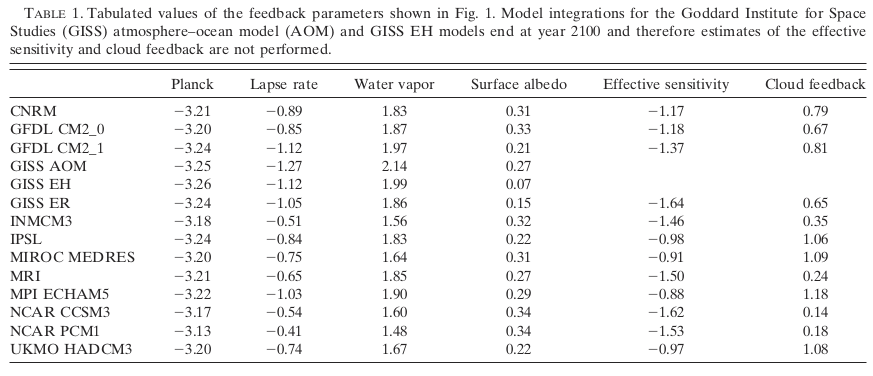
For completeness, here is the S&H table of the feedbacks:



Update. MarkR asked if I could post part of Fig 2. I think it is all quite interesting. Here it is, in two parts: