This is an ongoing topic of blog discussion - recently
here. I have written a few posts about it (eg
here), and there is an interactive gadget for seawater buffering
here. One of my themes is to reduce the emphasis on pH. The argument is that it is present in very small quantity; the buffering inhibits change, and so it is not a significant reagent. Because of its sparsity, it was until recently hard to measure. So both with measurement and conceptually, it is better to concentrate on the main reagents. These are CO₂, bicarb HCO₃⁻ and carbonate CO₃⁻². Carbonate is also involved in a solubility equilibrium with CaCO₃.
There is resistance to defocussing on H⁺, based on older notions that it is the basis of acidity. But for 95 years we have had the concept of
Lewis acidity, in which a proton is just one of many entities that can accept an electron pair. CO₂ is another such Lewis acid. And to it makes possible the description of the
overall reaction of CO₂ absorption
CO₃⁻² + CO₂ + H₂O ⇌ 2HCO₃⁻
as a Lewis acid/base reaction, in which carbonate donates an electron pair to CO₂. I propound that, but meet resistance from people who think Lewis acidity is an exotic modern concept.
I've realised now that that isn't necessary, because the notion of buffering isn't tied to any notion of acidity. So I can set up buffer equations just involving those three major reagents.
pH Buffer
A buffer is
normally described as an equilibrium
A + H ⇌ HA
where HA is a weak acid, A the conjugate base and H a proton. I have dropped the charge markings. The system operates as a buffer as long as substantial concentrations of both A and HA are present. I'll denote concentrations as h, a and ha.
The maths of the buffer system comes from the equations
| h*a/ha = K | (M) |
| ha + h = cH | (H) |
| ha + a = cA | (A) |
Eq (M) is the
Law of Mass Action. Eq (H) is mass balance of H, and (A) of A. As the reactions of the equilibrium proceed, the numbers on the right are invariant within the reactions. The equilibrium will shift if one of them changes from outside effect.
The equations are a mixture of multiplicative and linear, and in the
buffer calculator I used a Newton-Raphson method to solve the coupled systems. But for one buffer there is a simple way which illustrates the buffering principle. The iteration for given K, cH and CA goes:
starting with h=0
1 solve (H) and (A) for a and ha
2 solve (M) for h and repeat (if really necessary)
Under buffer conditions K is small, and so is H, and so changing h will not make much relative change to ha and a, and so in turn will not affect the next iteration of h that emerges from solving (M). The process converges quickly and ensures h stays small. The buffer is perturbed by changing cH or cA, either by adding reagents or by perturbing other equilibria in which reagents are involved. Eq (M) ensures that h not only remains small, but is fixed by the slowly changing ratios of the major species.
Here is a worked example. A litre of 1M A, 1M HA, pKa=8 (so pH=8).
Add 0.1M HCl, sufficient to reduce pH of water to 1.
Then, ignoring volume change:
ha=1.1 (eq H, total H) and ha+a=2 (eq A) so a=0.9.
Then from (M), h=1e-8*1.1/0.9=1.222e-8
On iteration, the corrections to (H) and (A) would be negligible. The pH has gone from 8 to 7.91
Now there is no mention of any kind of acidity in this math. The only requirement is that there is a ternary equilibrium in which one component H is in much lower concentration than the others. H could be anything So I didn't need to talk about Lewis acids (it helps understanding but not the buffer math).
Bjerrum plot
The classic way of graphing buffer relations is with a
Bjerrum plot. This takes advantage of the fact that you can divide a and ha by cA, and eq (M) is not changed. Eq H would be, but you can let it go if h is specified as the x-axis variable. Then M is solved to show a/cA and ba/cA (which add to 1) as functions of h, or usually, -log10(h). Actually, Bjerrum plots are really only interesting for coupled equilibria. Here is a Wiki example:

Generalised buffer - sea water
Sea water buffering is complicated, in normal description, by the interaction of two pH buffers (numbers from
Zeebe)
| HCO₃⁻+H⁺ ⇌ CO₂ + H₂O | K1: pKa=5.94 |
| CO₃⁻²+H⁺ ⇌ HCO₃⁻ | K2: pKa=9.13 |
The pKa for a H,A,HA buffer is the pH at which ha=a. K1, K2 are the equilibrium constants, as in Eq (M). So it is a complicated calculation. But the two can be combined, eliminating the sparse component H⁺, as before
CO₃⁻² + CO₂ + H₂O ⇌ 2HCO₃⁻
Now we still have an essentially ternary equilibrium, since the concentration of water does not change. And [CO₂] is still small. It is essentially a buffer equation, but buffering [CO₂]. The equations now are, with A=CO₃⁻², HA=HCO₃⁻ and H=CO₂:
| h*a/ah² = K | (M') |
| ha + a + h = cC | (C) |
| ha + 2*a = cE | (E) |
The additive equations are different; I've renamed them as (C) (total carbon, or dissolved inorganic carbon cC=DIC) and (E) (cE = total charge, or total alkalinity TA). K can be derived from the component buffers above, K=K2/K1, so -Log10(K) = 9.13-5.94 = 3.19
Summarising for the moment:
-
I have replaced two coupled acid/base buffers with a single equilibrium with buffering properties, eliminating H⁺.
- The components are the main carbonate reagents, which we can solve for directly.
- The additive equations conserve the measurement parameters DIC and TA.
- CO₂ replaces H⁺ as the sparse variable, and also the measure of (Lewis) acidity.
Bjerrum plot for generalised buffer
This uses the same idea of choosing a x-axis variable, and using the equation that results from eliminating it from the additive equations as the constraint, scaling wrt its rhs. The x-axis here uses the scarce species H=CO₂, and the eq (E) for total alkalinity is suitable for normalising, since cE=TA does not change as h varies. So the new plot variables are
- x = -log10(h/cE)
- y = 2*a/cE
- y'=1-y=ha/cE
Here is the plot, using
standard concentrations a=260, ha=1770 μM, K=K2/K1=6.46e-04, so TA=2290 μM
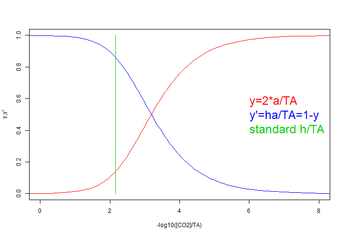
For the simple pH buffer, the curves would be tanh functions; here they are similar but not symmetric. More acid solutions are to the left; the green line represents equilibrium h for those conditions; adding CO₂ does not change the normalising TA and moves the green line to the left.
Perturbing an equilibrium by forcing concentration
Again a natural iteration can be used for the equations, based on the small component. However, in the real OA problem, we don't add a finite amount of reagent, but force an new change in the buffered quantity [CO₂] by air change. Then the buffering effect works in reverse; a small change forces big changes elsewhere.
Suppose we have a pond of seawater, with
standard concentrations a=260, ha=1770, h=[CO₂]=10 μM. Suppose the pCO₂ in air rises by fraction f. We don't actually need to know what pCO₂ is, just use Henry's law to say [CO₂] will increase in the same ratio. We can't use eq (C), because change in cC is unknown, but eq (E) says Δha = -Δa. Letting x be the fractional change in a, and m=2*a/ha=0.294, so the fractional change in ha is -m*x so from (M') we have,
(1+f)*(1+x)/(1-m*x)² = 1 (ratio change)
or f+x*(1+f+2*m) = (m*x)² (ratio change)
We could solve this as quadratic, but it is instructive to iterate, solving
x<- -(f-(m*x)²)/(1+f+2*m) starting with x=2
With f=0.1 (10%) the iterates are -0.07175, -0.07166737, -0.07166755
The first term is good enough. The key result is that a 10% change in atmospheric CO2 makes a 7% change, at equilibrium, with [CO₃⁻²], even though its concentration remains very small. Note that there is no reference to pH in this calculation. pH can be recovered from eq (M).
Repeating that main result; if m=[CO₃⁻²]/[HCO₃⁻] and the fractional change in gas phase pCO₂ is f, then the fractional change x in [CO₃⁻²] is given to very good approximation by
x = f/(1+f+2*m)
Estimates of m vary, but are usually around 0.1. So the fractional reduction in [CO₃⁻²] is comparable to the fractional increase in pCO₂.
Of course that is an equilibrium calculation, and the mixing time of the whole ocean is very long, so it could only apply to surface layers. It also omits the key question of CaCO₃ dissolution, which could restore [CO₃⁻²]. That dissolution is seen as the penalty, and this quantifies it.
Summarising again the virtues of this approach:
- It eliminates H⁺ and deals with the reagents directly
- The natural measures are the Dissolved Inorganic Carbon (DIC) and Total Alkalinity, both easily lab-measured and with data available
- It gives a useful approximation to the natural forcing condition, which is change in pCO₂ in the air
- The concept is that [CO₂] is buffered rather than pH. That leads directly to the consequence that trying to force a change in [CO₂] passes directly to a change in carbonate instead.