Wednesday, December 23, 2015

Merry Christmas - and a new kind of movie

Firstly I wish a Merry Christmas to all readers. Here is a picture of a local solstice scene:


What AGW can do for you! As mentioned, I've been dabbling with NOMADS systems, and downloading data from GFS. I showed here a conventional animation of relative humidity, as it is convected around the world.

Regular readers will know that I have a strong preference for using spherical projections, in conjunction with active viewing (Javascript). The most powerful way of doing this with movies is with WebGL. I rigged up a system here with high resolution SST, but it's rather slow, and not in good repair. The problem is that too much data needs to be downloaded with each frame. I don't think it's practical to preload a whole movie, though I haven't really tried.

So I thought to go back to a pre-WebGL (and HTML 5) system that I had with displaying ordinary graphics files, as here. You can look at the world from a few viewpoints, typically faces of a Platonic solid. So in this movie, it's the faces of a cube - ie six views, 2 polar, 4 equator. Use the radio buttons to switch. It's again of surface relative humidity - this time of 33 days, starting November 11. It's GFS data from NOAA NOMADS, on a 0.5° grid. Below the fold.

Tuesday, December 15, 2015

November GISS down by only 0.01° on record October.

As reader David Sanger noted November GISS global average is out, at 1.05°C anomaly. That would be the hottest in the record, if they had not increased October to 1.06°C. The late rise in Oct is not unexpected, since as Olof noted, Brazil and Greenland came in late and relatively warm. TempLS Oct went up too.

Most of the indices now agree on a very slight reduction from October to November. TempLS mesh is down 0.035°C; the NCEP/NCAR index was down about 0.05°. TempLS grid was down 0.01°C, and even the troposphere indices from satellite showed a similar small drop. TempLS mesh and GISS are generally more sensitive to polar changes, which were not large this time.

In other news, December is looking very warm indeed, in the NCEP/NCAR index. I had earlier written about a huge peak in early October, which made October a record month by a great margin. The peak of recent days is much larger again, almost reaching 1°C (1994-2013 base) and staying there for several days, though the latest reading was down to a mere 0.&°C. The average for December so far stands at 0.794°C, 0.23°C higher than October's record.

Even the sea ice is responding. Both Arctic and Antarctic are well down.

Saturday, December 12, 2015

A chaotic process, and climate analogy.

In my previous post, I described an article at WUWT called A simple demonstration of chaos and unreliability of computer models. It claimed issues about solving a simple differential equation which cast general doubt on the reliability of models, but in fact was using iterations far to large to say anything sensible about the DE.

But the recurrence does, for large parameter, generate a chaotic sequence which has useful analogies to waether, climate and their emulation. Here is a plot of part of that sequence. The green, red and blue points are initially separated by a distance of 0.0001 K. The recurrence starts at T0=300K, and follows the sequence
Tn+1=Tn+b*(1-(Tn/Te)4)         Te=243K, b=170
I follow three sequences, red starting at T0=300K (red), with green and blue separated there from red by 0.0001 K.

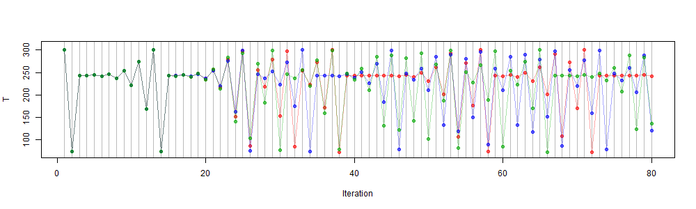
They are initially indistinguishable, but start to separate after about 25 iterations, and although they then sometimes come together, after about 50 timeteps there is really no association between them. You can't usefully predict where any starting point will lead to at that time, because the differences in those initial values are unlikely to be measurable. In fact, as I indicated in the last post, the growth in separation is initially exponential, so the slightest difference in floating value, say 1e-12, will lead to separation delayed by only another thirty or so iterations. I'll give much more detail about this process below.

Weather forecasting is similar. An initial state can be measured with finite accuracy, but small discrepancies grow, so the calculated forecast is useful for only about ten days at most. There is every reason to believe that the Earth itself has a corresponding magnification of small changes. So a perfect emulator could still not predict.

However, some things can be said. The plot remains within finite bounds, the same for each color. You can see that there are patterns whereby sequences of temperature around T0 are frequent. I will show histograms of frequency of temperatures, which are strongly patterned, and the same for each trajectory. These are the "climate", which is what can be determined in the presence of chaos. And they apply independent of starting points. Finding them is a boundary value problem, not an initial value problem.

I will also show that the climate is quite dependent on the parameter b, and that its dependence can be reliably determined from solution sequences, analogous to GCM runs.

Wednesday, December 9, 2015

Differential equations gone wrong

There was a post at WUWT called A simple demonstration of chaos and unreliability of computer models. It puported to solve a simple problem of a radiating black body coming to equilibrium with an internal heat source. But it was formulated as a non-linear recurrence relation. Some chaotic behaviour was demonstrated, but mis-attributed to methods of evaluating powers, and floating point issues.

I commented, first taking issue with the foolishness of this line of posting which quotes a simple and easily solved issue to say that there is something wrong with computer models in general. By which they mean, of course, climate models, but the alleged problem is quite generic. If the proposition were accepted, large areas of much-used engineering maths would have to be abandoned. Which is nonsense. David Evans claiming some issue about partial derivatives was another example. Also Hans Jelbring.

I went on to talk about the fact that the recurrence relation did not at all solve the underlying differential equation (DE). I made reference to stiff differential equations and suggested ways in which this could be improved. In a way, this missed the mark, because the author had never formulated it as a de. He just wrote down the recurrence for what was a very large time step, and found fault with it. But the recurrence does not in itself describe any real physics. It only does so insofar as it provides approximate solutions to the differential equation which does represent the process. And in his case, it certainly didn't. Because of the excessive timestep, the solutions were oscillatory, instead of the proper exponential approach to equilibrium. In one case, there was still convergence, in the other not. The latter case did show chaotic behaviour, where he got lost with red herrings about floating point and how powers are calculated. This was reflected in the discussion. In fact, the relevant maths is the magnification of small differences, which is the key point of chaos. The source of the differences is immaterial. But the magnification is already present in the linearised equation.

So in this post, I'll talk more about the differential equations aspect. Posters at WUWT frequently have no concept of what is involved in numerical DE. But there was also a real chaos problem. It's not connected with any physics here, but it is an example of the same kind as the standard quadratic recurrence, often related to predator-prey, and described at WUWT here. I think I can use this as a useful example of the chaotic aspect of climate modelling - how dependence on initial conditions fails, but this doesn't affect the ability to model climate. That will be Part 2 (probably more interesting).

Tuesday, December 8, 2015

TempLS November, down .04°C from October, but very warm.

There are now more than 4000 stations reporting for November. TempLS mesh estimated the global temperature anomaly at 0.88°C, down from 0.922 in October. It is still a lot higher than any other month in the record (0.76°C in Jan 2007). TempLS grid was very similar. The report is here.

The result is in line with the Moyhu NCEP/NCAR index, which dropped by about 0.05°C, but again exceeded any other month by about 0.1°C.

There was warmth in Europe, N America (except western US) and Brazil. Cool around Mongolia and N Atlantic. More detail in the WebGL plot. This month, most land areas contributed equally, to the anomaly, along with a small rise in SST.

Since this month NCEP and TempLS mesh and grid seem to be in agreement, it seems likely that other indices will follow. GISS was 1.04°C in October, so whether it will exceed 1 is a near thing. I'd say likelier than not.

In other news, the weekly OiSST NINO measures seem to be just below their peak levels. The satellite indices were down slightly. However, NCEP in December has been high, and the forecast is looking very warm.


Sunday, December 6, 2015

Big UAH adjustment.

I noticed in Roy Spencer's latest post the following observation:
Of course, everyone has their opinions regarding how good the thermometer temperature trends are, with periodic adjustments that almost always make the present warmer or the past colder.
It's true that adjustments at his UAH are less frequent. But when they happen, they are large. I decided to plot adjustments to UAH in this year, compared to the adjuatments in GISS (thermometer land/ocean) made over four years. The GISS version of Dec 2011 was the earliest I could find on the wayback machine. UAH brought out v6 in beta during 2015, replacing v5.6, which is however still maintained.

Update. I have found on wayback more GISS data going back to 2005 (the directory name had changed). I won't add it to the original graph; it is too close to the other GISS to show. I've added below the fold a graph of differences between each dataset, new minus old, to show adjustments on a better scale. The accumulation of 10 years of "periodic adjustments" to GISS is still dwarfed by the adjustment made to UAH in 2015.

I've set GISS to the UAH anomaly base, 1981-2010, and smoothed the monthly data with a running 12-month mean. I've used reddish for UAH, and blue for GISS.
Update: I have appended a plot including GISS 2015 an RSS, with better scaling, below.


AS you see, GISS adjustments are much smaller. I should mention that if you use the GISS base of 1951-1980 the adjustments look larger. The reason is that GISS is a much longer record, and adjustments are cumulative, and the earlier base period brings in all the adjustments since 1951.

Eli has a forceful critique of UAH here. Measurement by satellite interpretation of a very indirect signal in a place that is hard to locate exactly is always going to be chancy. As Dr Mears, the man behind the RSS satellite measure, said, in discussing measurement errors:
A similar, but stronger case can be made using surface temperature datasets, which I consider to be more reliable than satellite datasets (they certainly agree with each other better than the various satellite datasets do!).
His comment on agreement was made before UAH v6, which improved the agreement, but not confidence in their stability. I suspect that UAH (and RSS) should adjust more often, but that it is not done because of the inherent uncertainty.
Difference plot below


Thursday, December 3, 2015

NCEP/NCAR November, cooler than Oct, but warmer than any earlier month.

The Moyhu NCEP/NCAR index for November was 0.513°C, down from October's 0.567°C, but easily ahead (by about 0.1°C) of any other month in the record.

The warmth first shown in the October index corresponded to the rise later shown in GISS, and I would expect similar behaviour here. On the GISS anomaly base, the November NCEP index was 1.04°C.