Well, this post suggests another method, using TempLS v2. TempLS was a program written last year, originally to provide alternative calculation of the main global temperature indices. It did that. It works on a different basis to most other such codes - instead of gridding anomalies, it fits a linear model to global temperatures by weighted least squares.
Version 2 extended this to fitting spatial variation parametrised by coefficients of basis functions, intended to be families of orthogonal functions like spherical harmonics. But the EOF's introduced by Eric Steig for the Antarctica analysis would do as well.
This post describes some preliminary results. There are some loose parameters which will need better definition. I have done almost no verification stats. The trends come out rather high. But the patterns are quite similar to the O10/S09 results. And their are some big plusses. One is simplicity - run times are a few seconds instead of the 40+ minutes I found with the RO10 method. And the simplicity means that one can experiment with more things - eg spatial weighting.
Review of TempLS
There is a description of the math in V1 here. There is a general overview of stage 1 of the project here. You can find a complete listing of old posts (by category) at the Moyhu index. Incidentally, I've had to move the document repository recently, so if you have trouble finding online materials, the new location is hereThe math description of V2 is here. In V1, global temperatures were represented by the model:
The data has a number of stations (s), with temperature readings (x) by year (y) and month (m). m varies 1:12. Then x can be represented by a local temperature L, with a value for each station and month (seasonal average), and a global temperature G depending on year alone.
xsmy ~ Lsm + Gy
This is fitted by area-weighted least squares. The weight function w is an estimate of the inverse of the local density ofstations. The local temp L includes the variations due to station location, including seasonal effects, leaving G to represent global influences.
In V2 this modelling was extended to allow G to include spatial variation. As a computing trade-off, it was no longer allowed to vary freely with year. Instead, the part of interest here (model 2) required that it vary linearly with year, so the trend could be estimated.
The model is:
xsmy ~ Lsm + J yPsk Hk
Here J is a linear progression in y; P is a set of values of k basis functions at s locations, and H are the set of coefficients to be found. I'm using a summation convention, so summed over k. In the present context P can be the values of the satellite EOF's.
Ground station results
The natural starting point would be to take x as the set of ground station temperatures. There were 109 ground stations in total, 44 manned and 65 AWS. However, 5 were omitted in O10 for various reasons, and are omitted here. I also excluded stations above latitude 60S, although I forgot to include this in the count shown in the trend plots. The total was then 99.TempLS would normally weight by area density, but since AFAICT S09 and O10 did not do that, I won't either at this stage. The normal scheme based on lat/lon cells gets a bit messy. So here is the standard TempLS output - the map of stations and the graph of numbers of stations in each year. All the analysis will be from 1957-2006. You can right-click to see the small pics in full size.
 Map of ground stations  Numbers reporting |  Trends |
On the right is a plot made using Ryan's plot routine for consistency (and because it's good). At the top are indicated some parameters (more explanation soon), and the trends for the Continent, and for the Peninsula, West Antarctica, and East Antarctica (see map). The main parameter of importance at this stage is that 6 EOFs were used.
Comparison
Here are some results described on Ryan's post, and from Eric at RealClimate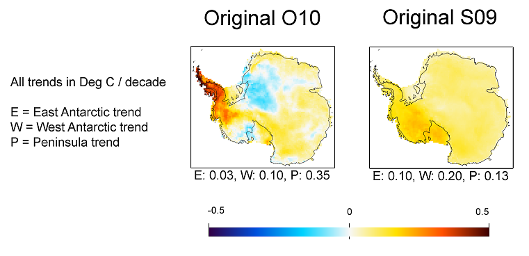 From Ryan's post 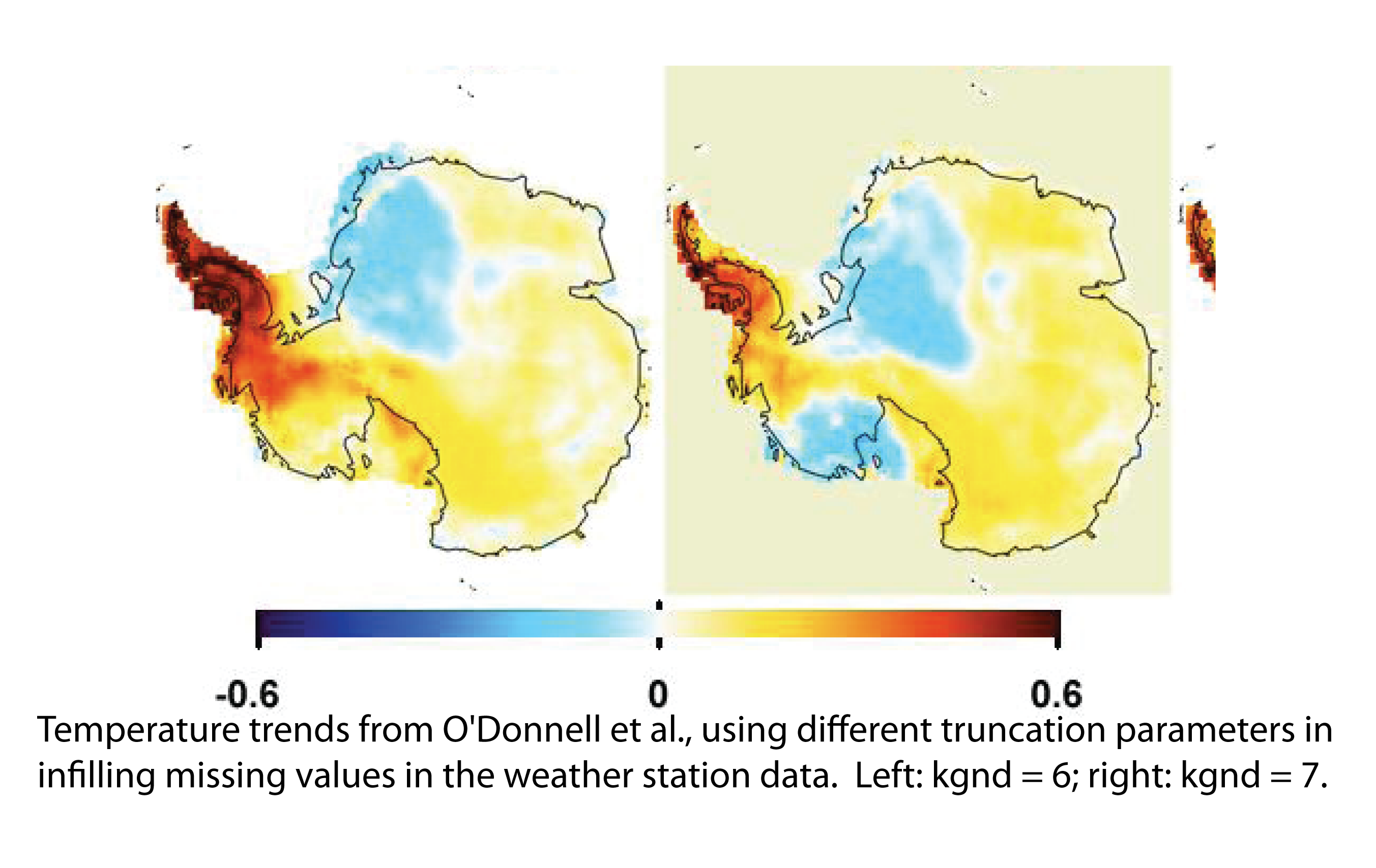 from Eric at RealClimate |
The TempLS pattern looks quite like O10's, but with larger trends in both directions. In the comparison, the continental trend was 0.06 for O10, and 0.12 for S09. So this value of 0.10 is in between. The Peninsula value of 0.56 is higher than both, as is the WA value, and EA is lower than both. But remember, the analysis so far was ground stations only
Use of AVHRR data
A key part of both S09 and O10 was infilling using both ground and AVHRR data. TempLS doesn't do infilling, but the natural equivalent is to add in artificial stations with AVHRR data. This was done with land/ocean indices - artificial stations created with SST data.We have 5509 AVHRR grid points, which gives more than enough coverage density. I reduced by a factor of 4 (leaving out alternate rows and cols in the rectangular grid of cells), making about 1392 in total. Theer will need to be relative weighting to prevent the ground stations being swamped, but for the moment I'll show the AVHRR stations only:
 Map of AVHRR "stations"  Numbers "reporting" |  Trends |
Mixing ground and AVHRR data
Now it's time to combine the data sets. There's no problem doing that - they are all in the same listing. The issue is relative weighting. If we want ground stations and AVHRR to have a roughly equal influence post 1980 (when both are available), then it would be appropriate to upweight the groundstations by a factor of about 15 (or maybe more, since ground stations have missing values, AVHRR generally not). So here is that case: Map of AVHRR "stations" |  Trends |
Again a pattern somewhat like that of O10, but with higher trends everywhere. The continent trend of 0.18 C/decade is very high.
Now it's time to explain the parameters shown on the trend plots. First is the number of ground stations, and then the number of AVHRR grids (though due to an error in the output program, this was underreported by 5). Then the weight factor, which is actually the number of extra times the ground stations are weighted (so if 15 is displayed, ground stations are upweighted by a total factor of 16). Then the number of AVHRR EOF's used as the basis functions. Finally, on the next line the trend values are reported.
Different weightings
OK, so we can try different weightings. I tried weightings of 8 and 40: Upweighting of ground stations =8 |  Upweighting of ground stations =40 |
The upweighting by 40 gives a pattern quite similar to O10. But again the Peninsula and WA trends are much higher.
Varying number of PCs
I've retained 6 EOFs above. The considerations seem to be similar to the S09 method. 4-6 looks like a good range, with noise problems increasing above 6. Here are the variations at weight factor 40: 4 EOFs |  5 EOFs | |
 6 EOFs |  7 EOFs | |
 8 EOFs |  9 EOFs |  10 EOFs |
Update. Here are plots of eigenvalues for the NxN matrix that has to be solved to get the coefficients (N=# PCs). I've shown N=5,7,10. The condition number is the ratio of largest to smallest. The max value of 53 for N=10 is getting large, but not disastrous.
 |
What still needs to be done?
A lot. I've done virtually no verification stats. Some sort of cross-validation is needed to get an optimal value of the weighting parameterhere the cost of departing from that is not prohibitive; the calc is currently a few seconds. But it would complicate the code.
(That isn't very accurate. The Santer/Quenouille correction affects the estimated error, which I haven't ventured yet. It wouldn't change the results quoted, although a fuller accounting for autocorelation would.)
And I could implement area-weighting. It's a bit complicated because of the differential weighting of the stations by type.
Update 27 May 2011
Kenneth Fritsch has been studying individual time sequences and breakpoints, as in the comments below. I'll link his graphics here:

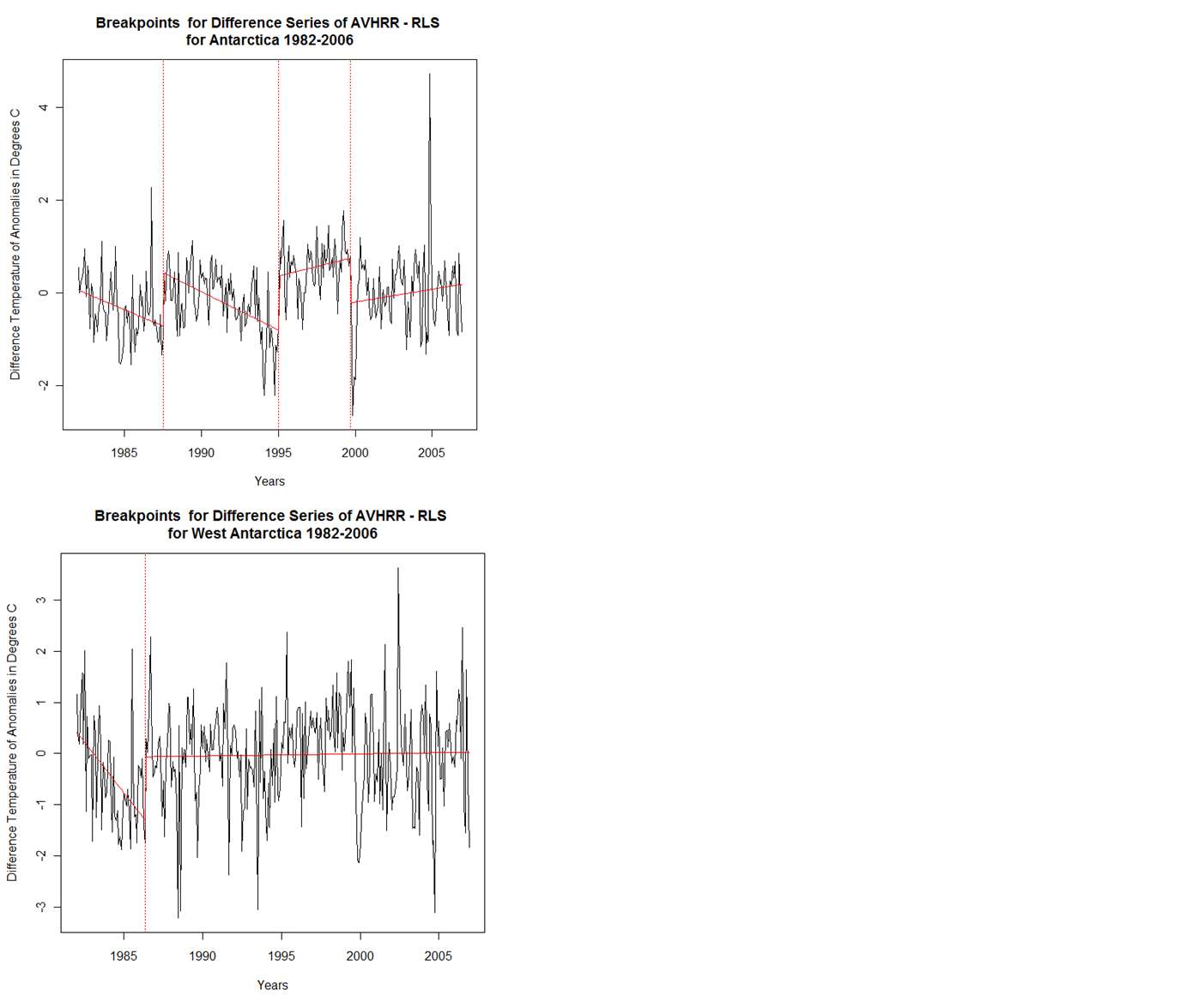


