Temperature averaging and integration - the basics

I write a lot about spatial integration, which is at the heart of global temperature averaging. I'll write more here about the principles involved. But I'm also writing to place in context methods I use in TempLS, which I think are an advance on what is currently usual. I last wrote a comparison of methods in 2015 here, which I plan to update in a sequel. Some issues here arose in a discussion at Climate Audit.

It's a long post, so I'll include a table of contents. I want to start from first principles and make some math connections. I'll use paler colors for the bits that are more mathy or that are just to make the logic connect, but which could be skipped.

• Basics - averaging temperature and integration
• Averaging and integration.
• Integration - theory
• Numerical integration - sampling and cells
• Triangular mesh
• Integration by function fitting
• Fitting - weighted least squares
• Basis functions - grid
• Basis functions - mesh
• Basis functions - spherical harmonics
• Basis functions - radial basis functions
• Basis functions - higher order finite element
• Next in the series.

Basics - averaging temperature.

Some major scientific organisations track the global temperature monthly, eg GISS, NOAA NCEI, HADCRUT 4, BEST. What they actually publish is global temperature average anomaly, made up of land station measurements and sea surface temperatures. I write often about anomalies, eg here. They are data associated with locations, formed by subtracting an expected value for the time of year. Anomalies are averaged; it isn't an anomaly of an average - a vital distinction. Anomalies must be created before averaging.

I also do this, with TempLS. Global average anomaly uses two calculations - an average over time, to get normals, and an average of anomalies (using normals) over space (globe). It's important that the normals don't get confounded with global change; this is often handled by restricting the anomaly to a common base period, but TempLS uses an iterative process.

Averaging and integration.

People think of averaging as just adding N numbers and dividing by N. I often talk of weighted averaging - Σ wₖxₖ / Σ wₖ (x data, w weights) Dividing by the weights ensures that the average of 1 is 1; a more general way of implementing is just to divide by trhe result of applying what you did to x to 1.

But the point of averaging is usually not to get just the average of the numbers you fed in, but an estimate of some population mean, using those numbers as a sample. So averaging some stations over Earth is intended to give the mean for Earth as a whole, including the points where you didn't measure. So you'd hope that if you chose a different set of points, you'd still get much the same answer. This needs some care. Just averaging a set of stations is usually not good enough. You need some kind of area weighting to even out representation. For example, most data has many samples in USA, and few in Africa. But you don't want the result to be just USA. Area-weighted averaging is better thought of as integration.

Let me give an example. Suppose you have a big pile of sand on a hard level surface, and you want to know how much you have - ie volume. Suppose you know the area - perhaps it is in a kind of sandpit. You have a graduated probe so that you can work out the depth at points. If you can work out the average depth, you would multiply that by the area to get the volume. Suppose you have a number of sample depths, perhaps at scattered locations, and you want to calculate the average.

The average depth you want is volume/area. That is what the calculation should reveal. The process to get it is numerical integration, which I'll describe.

Integration - theory

A rigorous approach to integration by Riemann in about 1854 is often cited. He showed that if you approximated an integral on a line segment by dividing it into ever smaller segments, not necessarily of equal size, and estimated the function on each by a value within, then the sum of those contributions would tend to a unique limit, which is the integral. Here is a picture from Wiki that I usd to illustrate. The idea of subdividing works in higher dimensions as well, basically because integration is additive. And the key thing is that there is that unique limit. Numerically, the task is to get as close to it as possible given a finite number of points. Riemann didn't have to worry about refined estimation, because he could postulatie an infinite process. But in practice, it pays to use a better estimate of the integral in each segment.

Riemann dealt with analytic functions, that can be calculated at any prescribed point. With a field variable like temperature, we don't have that We have just a finite number of measurements. But the method is the same. The region should be divided into small areas, and an integral estimated on each using the data in it or nearby.

The key takeaway from Riemann theory is that there is a unique limit, no matter how the region is divided. That is the integral we seek, or the volume, in the case of the sand pile.

Numerical integration - sampling and cells

The idea of integation far predates Riemann; it was originally seen as "antiderivative". A basic and early family of formulae is called Newton-Cotes. Formulae like these use derivatives (perhaps implied) to improve the accuracy of integration within sub-intervals. "Quadrature points" can be used to improve accuracy (Gauss quadrature). But there is an alternative view more appropriate to empirical data like temperature anomaly which is of inferring from sample values. This acknowledges that you can't fully control the points where function values are known.

So one style of numerical integration, in the Riemann spirit, is to divide the region into small areas, and estimate the integral of each as that area times the average of the sample values within. This is the method used by most of the majors. They use a regular grid in latitude/longitude, and average the temperatures measured within. The cells aren't equal area because of the way longitudes gather toward the poles; that has to be allowed for. There is of course a problem when cells don't have any measures at all. They are normally just omitted, with consequences that I will describe. GISS uses a variant of this with cells of larger longitude range near the poles. For TempLS, it is what I call the grid method. It was my sole method for years, and I still publish the result, mainly because it aligns well with NOAA and HADCRUT, also gridded.

Whenever you average a set of data omitting numbers representing part of the data, you effectively assume that the omitted part has the same behaviour as the average of what you included. You can see this because if you replaced the missing data with that average, you'd get the same result. Then you can decide whether that is really what you believe. I have described here how it often isn't, and what you should do about it (infilling). Here that means usually that empty cells should be estimated from some set of nearby stations, possibly already expressed as cell averages.

This method can be re-expressed as a weighted sum where the weights are just cell area divided by number of datapoints in cell, although it gets more complicated if you also use the data to fill empty cells (the stations used get upweighted).

While this method is usually implemented with a latitude/longitude grid, that isn't the best, because there is a big variation in size. I have explored better grids based on mapping the sphere onto a gridded Platonic polyhedron - cube or icosahedron. But the principle is the same.

Triangular mesh

My preferred integration has been by irregular triangular mesh. This recent post shows various meshes and explores how many nodes are really needed, but the full mesh is what the usual TempLS reports are based on. The msh is formed as a convex hull, which is what you would get if you drew a thin membrane over the measuring points in space. For the resulting triangles, there is a node at each corner, and to the values there you can fit a planar surface. This can be integrated, and the result is the average of the three values times the area of the triangle. When you work out the algebra, the weight of each station reading is the area of all the triangles that it is a corner of.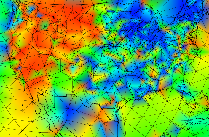

Integration by function fitting

There is a more general way of thinking about integration, with more methods resulting. This is where the data is approximated by a function whose integral is known. The usual way of doing this is by taking a set of basis functions with known integral, and linearly combining them with coefficients that are optimised to fit.

You can think of gridding as a special case. The functions are just those that take constant value 1 on the designated areas. The combination is a piecewise constant function.

Fitting - weighted least squares

Optimising the coefficients means finding ones that minimise s a sum of squares of some kind of the differences between the fit function and observed - called residuals. In math, that is
S = Σ wₖrₖrₖ where residual rₖ = yₖ-Σ bₘfₘ(xₖ)
Here yₖ and xₖ are the value and location; fₘ are the basis functions and bₘ the coefficients. Since there are usually a lot more locations than coefficients, this can't be made zero, but can be minimised. The weights w should again, as above, generally be area weights appropriate for integration. The reason is that S i a penalty on the size of residuals, and should generally be uniform, rather than varying with the distribution of sampling points.

By differentiation,
∂S/∂bₙ=0= Σₖ Aₖₙwₖ(yₖ-ΣₘAₖₘbₘ) where Aₖₙ=fₙ(xₖ)
or Σₘ AAₘₙ bₘ = Σₖ Aₖₙyₖ, where AAₘₙ = Σₖ AₖₘAₖₙ
In matrix notation, this is AA* b = A*y, where AA = A^TA
So AA is symmetric positive definite, and has to be inverted to get the coefficients b. In fact, AA is the matrix of scalar products of the basis functions. This least squares fitting can also be seen as regression. It also goes by the name of a pseudo-inverse.

This then determines what sort of basis functions f should be sought. AA ia generally large, so for inversion should be as well-conditioned as possible. This means that the rows should be nearly orthogonal. That is normally achieved by making AA as nearly as possible diagonal. Since AA is the matrix of scalar products, that means that the basis functions should be as best possibe orthogonal relative to the weights w. If these are appropriate for integration, that means that a good choice of functions f will be analytic functions orthogonal on the sphere.

I'll now review my various kinds of integration in terms of that orthogonality

Basis functions - grid.

As said above, the grid basis functions are just functions that are 1 on their cells, and zero elsewhere. "Cell" could be a more complex region, like combinations of cells. They are guaranteed to be orthogonal, since they don't overlap. And within each cell, the simple average creates no further interaction. So AA is actually diagonal, and inversion is trivial.

That sounds ideal, but the problem is that the basis is discontinuous, whereas there is every reason to expect the temperature anomaly to be continuous. You can see how this is a problem, along with missing areas, in this NOAA map for May 2017:



I described here a method for overcoming the empty cell problem by systematically assigning neighboring values. You can regard this also as just carving up those areas and adjoining them to cells that do have data, so it isn't really a different method in principle. The paper of Cowtan and Way showed another way of overcoming the empty cell problem.

Basis functions - mesh.

In this case, the sum squares minimisation is not needed, since there are exactly as many basis functions as data, and the coefficients are just the data values. This is standard finite element method. The basis functions are continuous - pyramids each with unit peak at a data point, sloping to zero on the opposite edges of the adjacent triangles. This combination of a continuous approximation with a diagonal AA is why I prefer this method, although the requirement to calculate the mesh is a cost. You can see the resulting visualisation at this WebGL page. It shows a map of the mesh approximation to TempLS residuals, for each month back to 1900.

Basis functions - spherical harmonics.

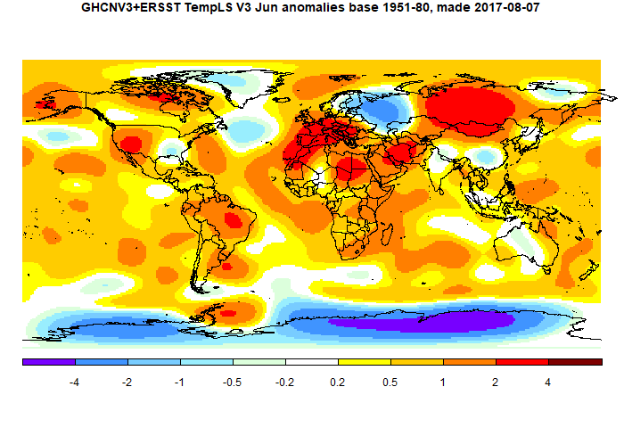
This has been my next favorite method. Spherical harmonics (SH) are described here, and visoalised here. I compared the various methods in a post here. At that stage I was using uniform weights w, and even then the method performed quite well. But it can be improved by using weights for any integration method. Even simple grid weights work very well. After fitting, the next requirement is to integrate the basis functions. In this case it is simple; they are all zero except for the first, which is a constant function. So for the integral, all you need is the first coefficient.

I also use the fit to display the temperature field with each temperature report. SH are smooth, and so is the fit. Here is a recent example:



This is the first case where we have a non-trivial AA to invert. I tend to use 100-200 functions, so the matrix can be inverted directly, and it is very quick in R. For a bigger matrix I would use a conjugate gradient method, which would be fine while the matrix is well-conditioned.

But it is conditioning that is the limitation. The basis functions have undulations, and at higher order, these start to be inadequately resolved by the spacing of data points. That means that, in terms of the approximate integration, they are no longer nearly orthogonal. Eventually AA becomes nearly singular, which means that there are combinations that are not penalised by the minimising of S. These grow and produce artefacts. SH have two integer parameters l and m, which roughly determine how many periods of oscillation you have in latitude and longitude. With uniform w, I can allow l up to 12, which means 169 functions. Recently with w right for grid integration, I can go to 16, with 289 functions, but with some indication of artefacts. I'll post a detailed analysis of this soon. Generally the artefacts are composed of higher order SH, so don't have much effcet on the integral.

Basis functions - radial basis functions.

This is a new development. RBFs are functions that are radially symmetric about a centre point, and fade from 1 toward 0 over a distance scaled to the spacing of data. They are smooth - I am using gaussians (normal distribution), although it is more common to use functions that go to zero in finite distance. The idea is that these functions are close to orthogonal if spaced so only their tails overlap.

It's not necessarily much different to SH; the attraction is that there is flexibility to increase the spread of the functions where data is scarce.

Basis functions - higher order finite element.

I used above the simplest element - linear triangles. There is a whole hierarchy that you can use with extra parameters, for example, quadratic functions on triangles with mid-side nodes. In these implementations, the mesh nodes will no longer be data nodes, so there is non-trivial fitting within elements. It is more complicated than, say, RBF. However there is a powerful technique in FEM called hp-fitting. Here the order of polynomial fit functions is increased as the size of the elements decreases. In theory there is a very rapid gain in accuracy, limited by discontinuity at boundaries, which we don't have. However, there is the problem of having to fit the polynomials within each element, so I don't know how that will work out.

Next in the series.

I've tried to lay out the theory in this post for reference. I'll do a post on more detail of spherical harmonics, calculating condition numbers and trying to optimise the weights and number of bases. I'll also do an updated post on a comparison of the methods. If RBFs really prove successful, I'll write about that too.