A short time ago, while writing about the discrepancy between the NCEP/NCAR index and TempLS mesh, I made a temporary modification to the daily WebGL plot to show monthly averages. I've now formalised this. There is a black bar at the top of the date selector, and if you mouseover that, it will offer monthly averages. They are all there now, including the current month (to date). I expect this will be kept up to date.
Monday, June 29, 2015
Friday, June 26, 2015
TempLS V3 - part 2
In my previous post, I began a three part description of the new vwrsion of TempLS. That part was devoted to the collection of land and SST data into a temperature data array.
The next part is about forming the other basic array for the calculation - the weighting array, with one entry for each temperature measurement. I've described in various posts (best summarized here) the principles involved. A spatial average (for a period if time, usually month) requires numerical spatial integration. The surface is divided into areas where the temperature anomaly can be estimated from data. If the subdivisions do not cover the whole area, the rest will be assumed (by the arithmetic) to have the average anomaly of the set that does have data. The integral is formed by adding the products of the estimates and their areas. That makes a weighted sum of the data.
The stage begins by loading saved data from the previous part. At this stage the land and SST data are concatenated, and a combined inventory made, from which the lat/lon of each station will be needed. R[] are filenames of saved data, consistent with the job control.
Then the choice is made (from the job, third char) between grid and mesh. We'll start with grid:
It's just a matter of assigning a unique number to each cell, and a vector with an entry for each of those numbers, and going through each month/year, counting. In R it is important to use fairly coarse-grained operations, because each command has an interpretive overhead.
Then continuing with the "else" part, for mesh weighting
This is more complicated. The mesh is actually the convex hull of the points on the sphere, which the R package alphahull calculates via convhulln(). This is quite time consuming (about 20 mins on my PC), so I save the results on a "w_.." file. So it reads the most recent, if any, and for months where the pattern of months matches, it uses the stored, which is much faster. Also the lat/lon of stations are converted to a unit sphere.
So we enter the ii loop over months with x and a w array waiting to be filled. If stored w doesn't match, the convex hull is formed. Then A, the areas are found. Note that convhulln does not consistently orient triangles, so the abs() is needed. The areas are in fact determinants, again calculated in a way to minimise looping.
Then it's just a matter of assigning area sums to nodes. This isn't so easy without fine looping, since each column of the m array of triangles has multiple occurrences of nodes. So in the jj loop, I identify a unique set of occurrences, add those areas to the node score, remove them, and repeat until all areas have been allocated. The last part just saves the newly calculated weights for future reference.
The last code in this step just saves the result for the calculation step 4.
Here is the complete code for this stage:
The next part is about forming the other basic array for the calculation - the weighting array, with one entry for each temperature measurement. I've described in various posts (best summarized here) the principles involved. A spatial average (for a period if time, usually month) requires numerical spatial integration. The surface is divided into areas where the temperature anomaly can be estimated from data. If the subdivisions do not cover the whole area, the rest will be assumed (by the arithmetic) to have the average anomaly of the set that does have data. The integral is formed by adding the products of the estimates and their areas. That makes a weighted sum of the data.
|
Traditionally, this was done with a lat/lon grid, often 5°×5°. An average is formed for each cell with data, in each month, and the averages are summed weighted by the cell area, which is proportional to the cosine of latitude. That is not usually presented as an overall weighted average, but it is. HADCRUT and NOAA use that approach. TempLS originally did that, so that the weight for each station was the cell area divided by the number of stations reporting that month in that cell. Effectively, the stations are allocated a share of the area in the cell.
Of course, this leaves some cells with no data. Cowtan and Way explored methods of interpolating these areas (discussed here). It makes a difference, because, as said, if nothing is done, those areas will be assigned the global average behaviour, from which they may in fact deviate. Recently, I have been using in preference an irregular triangular mesh (as shown right), of which the stations are the nodes. The weighting is made by assigning to each station a third of the area of each triangle that they are part of (see here). This has complete area coverage. I have continued to publish results from both the grid and mesh weighting. The code below shows how to form both kinds of weights. Note that the weighting does not use the actual measurements, only their existence. Stations with no result in a month get zero weight. There is no need for the weights to add to 1, because any weighted sum is always divided by a normalising sum. | 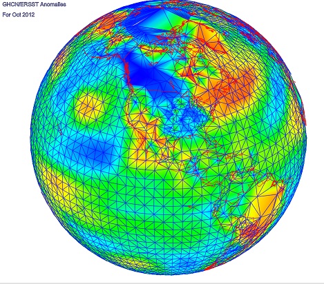 |
The stage begins by loading saved data from the previous part. At this stage the land and SST data are concatenated, and a combined inventory made, from which the lat/lon of each station will be needed. R[] are filenames of saved data, consistent with the job control.
if(do[3]){ #stage 3 -  wts from supplied x
 load(R[2])  # ERSST x,iv
 x0=x;i0=cbind(iv,NA,NA,NA,NA); rad=pi/180;
 load(R[1])  # GHCN x,iv
 colnames(i0)=colnames(iv)
 x=rbind(x,x0);iv=rbind(iv,i0)  # combine
Then the choice is made (from the job, third char) between grid and mesh. We'll start with grid:
 if(kind[3]=="g"){  #Grid
  dl=180/36 # 36*72 grid for wts
  jv=as.matrix(iv[,1:2])%/%dl # latlon integer number for each cell
  y=cos((jv[,1]+.5)*dl*rad)  #trig weighting for area each cell
  kv=drop(jv%*%c(72,1)+1297)  # Give each cell a unique number
  w=array(0,dim(x))
  for(i in 1:ncol(x)){  # over months
   j=which(!is.na(x[,i])) #  stations with data
   s=1/table(kv[j]) # stations in each cell
   u=as.numeric(names(s)) #cell numbers
   k1=match(kv[j],u) # which cell numbers belong to each stat
   w[j,i]=y[j]*s[k1]
  }
 }else{ # Mesh
It's just a matter of assigning a unique number to each cell, and a vector with an entry for each of those numbers, and going through each month/year, counting. In R it is important to use fairly coarse-grained operations, because each command has an interpretive overhead.
Then continuing with the "else" part, for mesh weighting
  require("geometry")
  require("alphahull")
  a=pc("w_",R[3])
  if(file.exists(a)){load(a)}else{w=array(0,dim(x))}  # old mesh
  a=cos(cbind(iv[,1:2],90-iv[,1:2])*rad)
  z=cbind(a[,1]*a[,c(2,4)],a[,3]) # to 3D coords
  if(!exists("w_yr"))w_yr=yr
  w=w[,mth(w_yr)%in%mth(yr)]
  if(sum(dim(w)==dim(x))<2){w=array(0,dim(x));}
  for(ii in 1:ncol(x)){
   o=!is.na(x[,ii]) # stations with data
   no=sum(o); if(no<9)next;  # skip months at the end
   if(sum(xor(o,(w[,ii]>0)))==0)next; # w slots match x, so use old mesh
   y=z[o,]
   m=convhulln(y) # convex hull (tri mesh)
   A=0
   B=cbind(y[m[,1],],y[m[,2],],y[m[,3],])
   for(j in 0:2){  # determinants for areas
    k=(c(0:2,0,2,1)+j)%%3+c(1,4,7)
    A=A+B[,k[1]]*B[,k[2]]*B[,k[3]]-B[,k[4]]*B[,k[5]]*B[,k[6]]
   }
   A=abs(A)  # triangles from convhulln have varied orientation
   n=cbind(c(m),rep(A,3)) # long list with areas matched to nodes
   k=which(o)
   w[!o,ii]=0
   w[o,ii]=1e-9  # to mark stations that missed wt but have x entries
   for(jj in 1:99){  # Adding areas for nodes
    i=match(1:sum(o),n[,1]) # find first matches in mesh
    q=which(!is.na(i))
    w[k[q],ii]=w[k[q],ii]+n[i[q],2]  # add in area
    n=rbind(n[-i[q],]) # take out matches
    if(length(n)<1)break;
   }
   print(c(ii,nrow(m),sum(w[,ii])/pi/24))
  } # end mesh months loop
This is more complicated. The mesh is actually the convex hull of the points on the sphere, which the R package alphahull calculates via convhulln(). This is quite time consuming (about 20 mins on my PC), so I save the results on a "w_.." file. So it reads the most recent, if any, and for months where the pattern of months matches, it uses the stored, which is much faster. Also the lat/lon of stations are converted to a unit sphere.
So we enter the ii loop over months with x and a w array waiting to be filled. If stored w doesn't match, the convex hull is formed. Then A, the areas are found. Note that convhulln does not consistently orient triangles, so the abs() is needed. The areas are in fact determinants, again calculated in a way to minimise looping.
Then it's just a matter of assigning area sums to nodes. This isn't so easy without fine looping, since each column of the m array of triangles has multiple occurrences of nodes. So in the jj loop, I identify a unique set of occurrences, add those areas to the node score, remove them, and repeat until all areas have been allocated. The last part just saves the newly calculated weights for future reference.
The last code in this step just saves the result for the calculation step 4.
 save(x,w,iv,file=R[3])
}#  end step 3
Here is the complete code for this stage:
if(do[3]){ #stage 3 -  wts from supplied x
 load(R[2])  # ERSST x,iv
 x0=x;i0=cbind(iv,NA,NA,NA,NA); rad=pi/180;
 load(R[1])  # GHCN x,iv
 colnames(i0)=colnames(iv)
 x=rbind(x,x0);iv=rbind(iv,i0)  # combine
 if(kind[3]=="g"){  #Grid
  dl=180/36 # 36*72 grid for wts
  jv=as.matrix(iv[,1:2])%/%dl # latlon integer number for each cell
  y=cos((jv[,1]+.5)*dl*rad)  #trig weighting for area each cell
  kv=drop(jv%*%c(72,1)+1297)  # Give each cell a unique number
  w=array(0,dim(x))
  for(i in 1:ncol(x)){  # over months
   j=which(!is.na(x[,i])) #  stations with data
   s=1/table(kv[j]) # stats in each cell
   u=as.numeric(names(s)) #cell numbers
   k1=match(kv[j],u) # which cell numbers belong to each stat
   w[j,i]=y[j]*s[k1]
  }
 }else{ # Mesh
  require("geometry")
  require("alphahull")
  a=pc("w_",R[3])
  if(file.exists(a)){load(a)}else{w=array(0,dim(x))}  # old mesh
  a=cos(cbind(iv[,1:2],90-iv[,1:2])*rad)
  z=cbind(a[,1]*a[,c(2,4)],a[,3]) # to 3D coords
  if(!exists("w_yr"))w_yr=yr
  w=w[,mth(w_yr)%in%mth(yr)]
  if(sum(dim(w)==dim(x))<2){w=array(0,dim(x)); }
  for(ii in 1:ncol(x)){
   o=!is.na(x[,ii]) # stats with data
   no=sum(o); if(no<9)next;  # skip months at the end
   if(sum(xor(o,(w[,ii]>0)))==0)next; # w slots match x, so use old mesh
   y=z[o,]
   m=convhulln(y) # convex hull (tri mesh)
   A=0
   B=cbind(y[m[,1],],y[m[,2],],y[m[,3],])
   for(j in 0:2){  # determinants for areas
    k=(c(0:2,0,2,1)+j)%%3+c(1,4,7)
    A=A+B[,k[1]]*B[,k[2]]*B[,k[3]]-B[,k[4]]*B[,k[5]]*B[,k[6]]
   }
   A=abs(A)  # triangles from convhulln have varied orientation
   n=cbind(c(m),rep(A,3)) # long list with areas matched to nodes
   k=which(o)
   w[!o,ii]=0
   w[o,ii]=1e-9  # to mark stations that missed wt but have x entries
   for(jj in 1:99){  # Adding areas for nodes
    i=match(1:sum(o),n[,1]) # find first matches in mesh
    q=which(!is.na(i))
    w[k[q],ii]=w[k[q],ii]+n[i[q],2]  # add in area
    n=rbind(n[-i[q],]) # take out matches
    if(length(n)<1)break;
   }
   print(c(ii,nrow(m),sum(w[,ii])/pi/24))
  } # end mesh months loop
  f=paste("w_",R[3],sep="") # for saving the wts if wanted
  w_yr=yr # save yrs to match when recalled
  if(!file.exists(f))save(w_yr,w,file=f)
 }# end mesh/grid
 save(x,w,iv,file=R[3])
}#  end step 3
Wednesday, June 24, 2015
TempLS: new V3
TempLS is my R program that I use for calculating global average temperatures. A recent review of the project is here. A few weeks ago I posted an iterative calculation sequence which is the basis of the program. I noted that the preliminaries for this were simple and mechanical. It requires the data just organised in a large array, and a set of weights, derived from station locations.
I've never actually released version 2.2 of TempLS, which is what I have been using. I did a documented release of v2.1 here. Meanwhile, the program continued to accumulate options, and got entwined with my automatic data acquisition system. So I thought it would be useful to create a simplified version with the basic functionality. I did post a simplified version once before, but that was land only, and with more primitive weighting.
So I'm planning to post a description with three parts. The first will be data gathering, the second weighting, and third is the calculation, which has already been covered. But there may be results to discuss. This is the first, which is about the data gathering. There is no fancy maths, and it is pretty boring, but useful for those who may use it.
The program is in four stages - GHCN, SST, weights and calc. The first two make up the data organising part, and are described here. Each stage stores its output, which the next reads, so can be run independently. I have a simple job control mechanism. You set a variable with four characters, the default is
job="UEGO"
There is one character for each stage; current provisions, according to location, are:
Each character can be lower case, which means skip that stage, but use the appropriate stored result. The point of this brevity is that the letters are used to name stored intermediate files, so the process can be re-started at any intermediate stage.
*** Note that ERSST has a new version V5, which I use. In this post, where I refer to V3b and V4, take it to be V4 and V5, including "job" above..
The program should be run in a dedicated directory - it will create subdirectories as needed. It starts with a section that defines some convenience functions, interprets the job code to make the names of the intermediate files (I use .sav for binary saved files), and defined the year range yr. This is hard-coded, but you can alter it.
Stage 1 begins with some function definitions, which I'll describe
It uses R facilities to download, unzip and untar. Then it finds the resulting files, data and inventory, which have a date-dependent name, and copies them into the current directory called ghcnu.dat etc. Then it removes the empty directory (else they accumulate). Download takes me about 30 secs. If you are happy with the data from before, you can comment out the call to this.
The next routine reads the data file into a big matrix with 14 rows. These are the station number, year, and then 12 monthly averages. It also reads the flags, and removes all data with a dubious quality flag. It returns the data matrix, converted to °C.
The rest is fairly simple:
The inventory is read, and the station numbers in d are replaced by integers 1:7280, being the corresponding rows of the inventory. iv is a reduced inventory dataframe; lat and lon are the first two columns, but other data is there for post-processing.
Then it is just a matter of making a blank x matrix and entering the data. The matrix emerges ns × nm, where ns is number of stations, nm months. Later the array will be redimensioned (ns,12,ny). Finally d and iv are saved to a file which will be called u.sav or a.sav.
So now we come to part 2 - SST. Here is how it starts:
ki is d,e for 3b,4; this is just making filenames for the cases. ERSST comes as a series of 89 x 180 matrices (2°), 10 years per file for 3b, and 1 year for v4. This is good for downloading, as you only have to download a small file for recent data. That is a grid of 16020 (some land), which is more than we need for averaging. SST does not change so rapidly. So I select just every second lat and lon. In v2.2 I included the missing data in a local average, but I'm not now sure this is a good idea. It's messy at boundaries, and the smoothness of SST makes it redundant. So here is the loop over input files
The files, when downloaded, are stored in a subdirectory, and won't be downloaded again while they are there. So to force a download, remove the file. I use cURL to download when there is a new version, but that requires installation. The first part of this code gathers each file contents into an array v. The -9999 values are converted to NA, and also anything less than -1°C. ERSST enters frozen regions as -1.8°C, but this doesn't make much sense as a proxy for air temperature. I left a small margin, since those are probably months with part freezing (there are few readings below -1 that are not -1.8).
Now to wrap up. A lat/lon inventory is created. Locations with less than 12 months data in total are removed, which includes land places. Then finally the data array x and inventory are stored.
So I'll leave it there for now. The program has the potential to create a.sav, u.sav, d.sav and e.sav, each with a data array x and an iv. A simple task, but in lines it is more than half the program. Stage 3, next, will combine two of these and make a weight array.
Here is the code presented here in one piece. It is stand-alone.
I've never actually released version 2.2 of TempLS, which is what I have been using. I did a documented release of v2.1 here. Meanwhile, the program continued to accumulate options, and got entwined with my automatic data acquisition system. So I thought it would be useful to create a simplified version with the basic functionality. I did post a simplified version once before, but that was land only, and with more primitive weighting.
So I'm planning to post a description with three parts. The first will be data gathering, the second weighting, and third is the calculation, which has already been covered. But there may be results to discuss. This is the first, which is about the data gathering. There is no fancy maths, and it is pretty boring, but useful for those who may use it.
The program is in four stages - GHCN, SST, weights and calc. The first two make up the data organising part, and are described here. Each stage stores its output, which the next reads, so can be run independently. I have a simple job control mechanism. You set a variable with four characters, the default is
job="UEGO"
There is one character for each stage; current provisions, according to location, are:
| U,A | Unadjusted or Adjusted GHCN |
| D,E | ERSST Ver 3b or V4 |
| G,M | Grid or mesh-based weighting |
| O,P | Output, without or with graphics |
Each character can be lower case, which means skip that stage, but use the appropriate stored result. The point of this brevity is that the letters are used to name stored intermediate files, so the process can be re-started at any intermediate stage.
*** Note that ERSST has a new version V5, which I use. In this post, where I refer to V3b and V4, take it to be V4 and V5, including "job" above..
The program should be run in a dedicated directory - it will create subdirectories as needed. It starts with a section that defines some convenience functions, interprets the job code to make the names of the intermediate files (I use .sav for binary saved files), and defined the year range yr. This is hard-coded, but you can alter it.
# Function TempLS3.r. Written in four stages, it collects data, makes weights
#and solves for global temperature anomaly.
#Written by Nick Stokes, June 24 2015.
#See  https://moyhu.blogspot.com.au/2015/06/templs-and-new-ersst-v4-noaa-is-now.html
#Functions
isin=function(v,lim){v>=lim[1] & v<=lim[2]}
mth=function(yr){round(seq(yr[1]+0.04,yr[2]+1,by=1/12),3)}
sp=function(s)(unlist(strsplit(s,"")))
pc=function(...,s=""){paste(...,sep=s,collapse=s)}
# Start program
if(!exists("job"))job="UEGO"
i=sp(job)
kind=tolower(i)
do=i!=kind
yr=c(1900,2015); yrs=yr[1]:yr[2]; # you can change these
ny=diff(yr)+1
j=c(1,1,2,2,1,3,1,4); R=1:4; #R will be the names of storage files
for(i in 1:4){ # make .sav file names
 R[i]=pc(c(kind[j[i*2-1]:j[i*2]],".sav"))
 if(!file.exists(R[i]))do[i]=TRUE; # if filename will be needed, calc
}
</=lim[2]}>
Stage 1 begins with some function definitions, which I'll describe
if(do[1]){  # Start stage 1 - read land (GHCN)
 getghcn=function(){ # download and untar GHCN
  fi="ghcnm.tavg.latest.qcu.tar.gz"
  fi=sub("u",ki,fi)  # switch to adjusted
  download.file(pc("https://www1.ncdc.noaa.gov/pub/data/ghcn/v3/",fi),fi);
  gunzip(fi,"ghcnv3.tar",overwrite=T);
  untar("ghcnv3.tar",exdir=".");
  di=dir(".",recursive=T)
  h=grep(pc("qc",ki),di,val=T) # find the qcu files un subdir
  h=grep("v3",h,val=T) # find the qcu files un subdir
  file.rename(h,Rr)
  unlink("ghcnm.*")
 }
It uses R facilities to download, unzip and untar. Then it finds the resulting files, data and inventory, which have a date-dependent name, and copies them into the current directory called ghcnu.dat etc. Then it removes the empty directory (else they accumulate). Download takes me about 30 secs. If you are happy with the data from before, you can comment out the call to this.
The next routine reads the data file into a big matrix with 14 rows. These are the station number, year, and then 12 monthly averages. It also reads the flags, and removes all data with a dubious quality flag. It returns the data matrix, converted to °C.
readqc=function(f){  # read the data file
 b=readLines(f)
 d=matrix(NA,14,length(b));
 d[1,]=as.numeric(substr(b,1,11));
 d[2,]=as.numeric(substr(b,12,15)); # year
 iu=0:13*8+4
 for(i in 3:14){
  di=as.numeric(substr(b,iu[i],iu[i]+4)); # monthly aves
  ds=substr(b,iu[i]+6,iu[i]+6); # quality flags
  di[ds!=" " | di== -9999]=NA  # remove flagged data
  d[i,]=di/100  # convert to C
 }
d
}
The rest is fairly simple:
 require("R.utils") # for gunzip
 ki=kind[1]  # u or a
 Rr=paste("ghcn",ki,c(".dat",".inv"),sep="")
 getghcn()
 d=readqc(Rr[1])
 b=readLines(Rr[2])
 ns=length(b)
 wd=c(1,11,12,20,21,30,1,3,31,37,88,88,107,107)
 iv=data.frame(matrix(NA,ns,6))
 for(i in 1:7){
  k=substr(b,wd[i*2-1],wd[i*2]);
  if(i<6 1="" airprt="" alt="" c="" colnames="" convert="" country="" d="" data="" dim="" each="" else="" end="" file="R[1])" fill="" for="" i-1="" i="=1)K=k" ib="match(d[1,],K)-1" ic="" if="" in="" iv="" k="as.numeric(k)" lat="" locations="" lon="" ns="" numbers="" ny="" of="" order="" place="" rearrange="" restrict="" row="" save="" stage="" station="" to="" urban="" x="" years="" yr="">
The inventory is read, and the station numbers in d are replaced by integers 1:7280, being the corresponding rows of the inventory. iv is a reduced inventory dataframe; lat and lon are the first two columns, but other data is there for post-processing.
Then it is just a matter of making a blank x matrix and entering the data. The matrix emerges ns × nm, where ns is number of stations, nm months. Later the array will be redimensioned (ns,12,ny). Finally d and iv are saved to a file which will be called u.sav or a.sav.
So now we come to part 2 - SST. Here is how it starts:
if(do[2]){ # Stage 2 - read SST
# ERSST has convention lon 0:358:2, lat -88:88:2
 ki=kind[2];
 s=c("ersst4","ersst.%s.%s.asc","ftp://ftp.ncdc.noaa.gov/pub/data/cmb/ersst/v4/ascii")
 iy=1;  if(ki=="d"){s=sub("4","3b",s);s[1]="../../data/ersst";iy=10;yrs=seq(yr[1],yr[2],10);}
 if(!file.exists(s[1]))dir.create(s[1])
 x=NULL; n0=180*89;
ki is d,e for 3b,4; this is just making filenames for the cases. ERSST comes as a series of 89 x 180 matrices (2°), 10 years per file for 3b, and 1 year for v4. This is good for downloading, as you only have to download a small file for recent data. That is a grid of 16020 (some land), which is more than we need for averaging. SST does not change so rapidly. So I select just every second lat and lon. In v2.2 I included the missing data in a local average, but I'm not now sure this is a good idea. It's messy at boundaries, and the smoothness of SST makes it redundant. So here is the loop over input files
    for(ii in yrs){
    # read and arrange the data
  f=sprintf(s[2],ii,ii+9)
  if(ki=="e")f=sprintf(s[2],"v4",ii)
  g=file.path(s[1],f)
  if(!file.exists(g))download.file(file.path(s[3],f),g);
        v=matrix(scan(g),nrow=n0);
  v=v[,(mth(c(ii,ii+iy-1)) %in% mth(yr))[1:ncol(v)]]/100  # Select years and convert to C
  n=length(v);
  o=v== -99.99 | v< -1  # eliminate ice -1
  v[o]=NA
  n=n/n0
  dim(v)=c(89,180,n)
  # reduce the grid
  i1=1:45*2-1;i2=1:90*2 # Take every second one
  v=v[i1,i2,]
  # normalise the result; w is the set of wts that were added
  x=c(x,v)
  print(c(ii,length(x)/90/45))
    }

</>
The files, when downloaded, are stored in a subdirectory, and won't be downloaded again while they are there. So to force a download, remove the file. I use cURL to download when there is a new version, but that requires installation. The first part of this code gathers each file contents into an array v. The -9999 values are converted to NA, and also anything less than -1°C. ERSST enters frozen regions as -1.8°C, but this doesn't make much sense as a proxy for air temperature. I left a small margin, since those are probably months with part freezing (there are few readings below -1 that are not -1.8).
Now to wrap up. A lat/lon inventory is created. Locations with less than 12 months data in total are removed, which includes land places. Then finally the data array x and inventory are stored.
 iv=cbind(rep(i1*2-90,90),rep((i2*2+178)%%360-180,each=45)) # Make lat/lon -88:88,2:358
 m=length(x)/90/45
 dim(x)=c(90*45,m)
 rs=rowSums(!is.na(x))
 o=rs>12  # to select only locations with more than 12 mths data in total
 iv=iv[o,] # make the lat/lon
 x=x[o,] #discard land and unmeasured sea
 str(x)
 ns=sum(o)  # number stations in this month
 rem=ncol(x)%%12
 if(rem>0)x=cbind(x,matrix(NA,ns,12-rem)) # pad to full year
 str(x)
 dim(x)=c(ns,12*((m-1)%/%12+1))
 save(x,iv,file=R[2])
} # End of stage 2
So I'll leave it there for now. The program has the potential to create a.sav, u.sav, d.sav and e.sav, each with a data array x and an iv. A simple task, but in lines it is more than half the program. Stage 3, next, will combine two of these and make a weight array.
Here is the code presented here in one piece. It is stand-alone.
# Function TempLS3.r. Written in four stages, it collects data, makes weights
#and solves for global temperature anomaly.
#Written by Nick Stokes, June 24 2015.
#See  https://moyhu.blogspot.com.au/2015/06/templs-and-new-ersst-v4-noaa-is-now.html
isin=function(v,lim){v>=lim[1] & v<=lim[2]}
mth=function(yr){round(seq(yr[1]+0.04,yr[2]+1,by=1/12),3)}
sp=function(s)(unlist(strsplit(s,"")))
pc=function(...,s=""){paste(...,sep=s,collapse=s)}
if(!exists("job"))job="UEGO"
i=sp(job)
kind=tolower(i)
do=i!=kind
yr=c(1900,2015); yrs=yr[1]:yr[2]; # you can change these
ny=diff(yr)+1
j=c(1,1,2,2,1,3,1,4); R=1:4; #R will be the names of storage files
for(i in 1:4){ # make .sav file names
 R[i]=pc(c(kind[j[i*2-1]:j[i*2]],".sav"))
 if(!file.exists(R[i]))do[i]=TRUE; # if filename will be needed, calc
}
if(do[1]){  # Stage 1 - read land (GHCN)
 getghcn=function(){ # download and untar GHCN
  fi="ghcnm.tavg.latest.qcu.tar.gz"
  fi=sub("u",ki,fi)  # switch to adjusted
  download.file(pc("https://www1.ncdc.noaa.gov/pub/data/ghcn/v3/",fi),fi);
  gunzip(fi,"ghcnv3.tar",overwrite=T);
  untar("ghcnv3.tar",exdir=".");
  di=dir(".",recursive=T)
  h=grep(pc("qc",ki),di,val=T) # find the qcu files un subdir
  h=grep("v3",h,val=T) # find the qcu files un subdir
  file.rename(h,Rr)
  unlink("ghcnm.*")
 }

readqc=function(f){  # read the data file
 b=readLines(f)
 d=matrix(NA,14,length(b));
 d[1,]=as.numeric(substr(b,1,11));
 d[2,]=as.numeric(substr(b,12,15)); # year
 iu=0:13*8+4
 for(i in 3:14){
  di=as.numeric(substr(b,iu[i],iu[i]+4)); # monthly aves
  ds=substr(b,iu[i]+6,iu[i]+6); # quality flags
  di[ds!=" " | di== -9999]=NA  # remove flagged data
  d[i,]=di/100  # convert to C
 }
d
}

 require("R.utils") # for gunzip
 ki=kind[1]
 Rr=paste("ghcn",ki,c(".dat",".inv"),sep="")
 getghcn()
 d=readqc(Rr[1])
 b=readLines(Rr[2])
 ns=length(b)
 wd=c(1,11,12,20,21,30,1,3,31,37,88,88,107,107)
 iv=data.frame(matrix(NA,ns,6))
 for(i in 1:7){
  k=substr(b,wd[i*2-1],wd[i*2]);
  if(i<6 -1="" -88:88:2="" -88:88="" -99.99="" -="" 0:358:2="" 2="" added="" airprt="" alt="" and="" arrange="" ascii="" b="" c="" cmb="" colnames="" convert="" country="" d="" data="" dim="" dir.create="" do="" download.file="" e="" each="" eliminate="" else="" ersst.="" ersst4="" ersst="" every="" f="" file.exists="" file.path="" file="R[1])" fill="" for="" ftp.ncdc.noaa.gov="" ftp:="" g="" grid="" has="" i-1="" i1="1:45*2-1;i2=1:90*2" i="=1)K=k" ib="match(d[1,],K)-1" ic="" ice="" if="" ii="" in="" is="" iv="cbind(rep(i1*2-90,90),rep((i2*2+178)%%360-180,each=45))" iy="10;yrs=seq(yr[1],yr[2],10);}" k="" ki="=" lat="" length="" locations="" lon="" m="" make="" mth="" n0="180*89;" n="" ncol="" normalise="" ns="" numbers="" ny="" o="rs" of="" one="" order="" place="" print="" pub="" read="" rearrange="" reduce="" restrict="" result="" row="" rs="rowSums(!is.na(x))" s.="" s.asc="" s="" save="" second="" select="" set="" sst="" stage="" station="" str="" take="" that="" the="" to="" urban="" v4="" v="v[i1,i2,]" w="" were="" wts="" x="" years="" yr="" yrs="">12  # to select only locations with more than 12 mths data in total
 iv=iv[o,] # make the lat/lon
 x=x[o,] #discard land and unmeasured sea
 str(x)
 ns=sum(o)  # number stations in this month
 rem=ncol(x)%%12
 if(rem>0)x=cbind(x,matrix(NA,ns,12-rem)) # pad to full year
 str(x)
 dim(x)=c(ns,12*((m-1)%/%12+1))
 save(x,iv,file=R[2])
}

</=lim[2]}></>
Sunday, June 21, 2015
TempLS and the new ERSST V4
NOAA is now using their new V4 ERSST, and so should I. It has come along at a time where I am preparing my own V3 of TempLS (more below), so I will make a double transition.
But first I should mention an error in my earlier processing of V3b, noted in comments here. ERSST3b came in decade files; that helped, because decades before the present did not change and did not require downloading. So I collected them into a structure, and with each update to the current decade (every month) merged that with the earlier decades.
However, I misaligned them. Most climate data uses the strict decade numbering (1961-90 etc), but ERSST uses 2000-2009. I got this wrong in the earlier data, creating a displacement by 1 year. Fixing this naturally gave better alignment with other datasets.
I'll describe the new TempLS version in detail in coming days. V 2.2 of TempLS had become unwieldy due to accumulation of options and special provisions for circumstances that arose along the way. I have made a new version with simplified controls, and using a simple iterative process described here. It should in principle give exactly the same answers; however I have also slightly modified the way in which I express ERSST as stations.
The new version is an R program of just over 200 lines. Of course, when simplifying there are some things that I miss, and one is the ability to make spherical harmonics plots (coming). So for a while the current reports will lag behind the results tabled above. That table, and the various graphs on the latest temperature page, will now be using ERSST v4.
Below the fold, I'll show just a few comparison results.
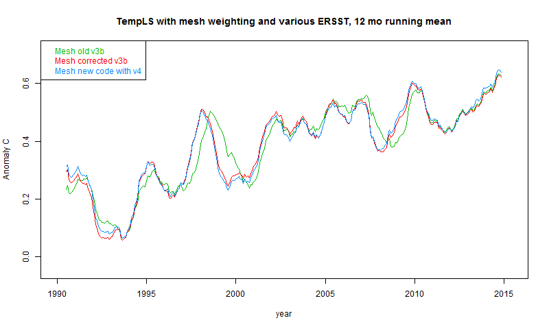
I've used running means to smooth out monthly noise, and focussed on the period since 1990. At some stage I might say more on the V4 changes, but that has been covered extensively elsewhere. I show the old results before fixing the missing year problem, then the V3b results after fixing, still using V2.2. Then there are results using new ERSS v4 and new TempLS V3. Ideally I would separate the effects of the new code and new ERSST, but getting V3b working with ERSST v4 would take a while, and the combined effect makes very little change.
So here are the grid weighted results. The effect of the year error is clear, but there is little change going from ERSST 3b and TempLS2.2 to ERSST 4 and TempLS 3.
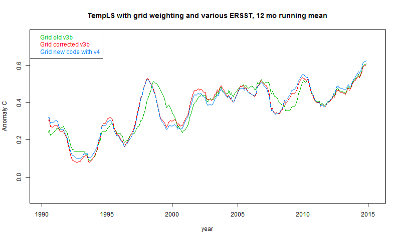
And here are the grid weighted results, which are similar.
But first I should mention an error in my earlier processing of V3b, noted in comments here. ERSST3b came in decade files; that helped, because decades before the present did not change and did not require downloading. So I collected them into a structure, and with each update to the current decade (every month) merged that with the earlier decades.
However, I misaligned them. Most climate data uses the strict decade numbering (1961-90 etc), but ERSST uses 2000-2009. I got this wrong in the earlier data, creating a displacement by 1 year. Fixing this naturally gave better alignment with other datasets.
I'll describe the new TempLS version in detail in coming days. V 2.2 of TempLS had become unwieldy due to accumulation of options and special provisions for circumstances that arose along the way. I have made a new version with simplified controls, and using a simple iterative process described here. It should in principle give exactly the same answers; however I have also slightly modified the way in which I express ERSST as stations.
The new version is an R program of just over 200 lines. Of course, when simplifying there are some things that I miss, and one is the ability to make spherical harmonics plots (coming). So for a while the current reports will lag behind the results tabled above. That table, and the various graphs on the latest temperature page, will now be using ERSST v4.
Below the fold, I'll show just a few comparison results.
I've used running means to smooth out monthly noise, and focussed on the period since 1990. At some stage I might say more on the V4 changes, but that has been covered extensively elsewhere. I show the old results before fixing the missing year problem, then the V3b results after fixing, still using V2.2. Then there are results using new ERSS v4 and new TempLS V3. Ideally I would separate the effects of the new code and new ERSST, but getting V3b working with ERSST v4 would take a while, and the combined effect makes very little change.
So here are the grid weighted results. The effect of the year error is clear, but there is little change going from ERSST 3b and TempLS2.2 to ERSST 4 and TempLS 3.
And here are the grid weighted results, which are similar.
Friday, June 19, 2015
New NOAA - record May anomaly
NOAA has a new version, based on the new ERSST4. This has prompted me to make a change in the NOAA data that I use. They publish two sets; I have been using MLOST, which is the traditional one based on 1961-90 anomalies. But they also publish a version based on 1901-2000, and this is what they use for their climate summary announcements. Updates to MLOST have been lagging, so it is time to change. The different basis shouldn't affect the usual plots on the latest data page, or the trendviewer, but will affect the tabulated numbers.
So the May number was considerably higher than the previous May, and as I expected, higher than April, unlike GISS. In fact, it was quite in line with the NCEP/NCAR index.
I see there is a post at WUWT suggesting that the new record is somehow an artefact of the new version. As I commented here, the versions differ very little in year to year changes, by month. It is very unlikely that the old version would not have shown a similar rise, and in both versions, May 2014 was hotter than any previous May.
Thursday, June 18, 2015
NCEP/NCAR matched to GISS, NOAA
In my previous post, I noted that comparing data on different anomaly bases brought in discrepancies because of vagaries of monthly averages over the base period. These are actually significant enough to detract from the use of the NCEP/NCAR index (base 1994-2013) in predicting GISS (1951-80) and NOAA (1961-90) indices.
So I have added to that table, below the NCEP monthly averages, recent monthly values adjusted to the earlier basis periods by adding the 1994-2013 month averages of GISS and NOAA anomalies. This expresses NCEP on those scales, although strictly, it is unique to those indices. Adding HADCRUT averages would give slightly different 1961-90 values.
I have also shown the actual GISS/NOAA values in the right column. The current tables are here:
Except for GISS May, the correspondence is very good.
Update. I calculated a whole lot more values, in a table below the fold. It looks as if the last few months aren't typical. The correspondence is still reasonable, but discrepancies as observed April-May are not unusual.
So I have added to that table, below the NCEP monthly averages, recent monthly values adjusted to the earlier basis periods by adding the 1994-2013 month averages of GISS and NOAA anomalies. This expresses NCEP on those scales, although strictly, it is unique to those indices. Adding HADCRUT averages would give slightly different 1961-90 values.
I have also shown the actual GISS/NOAA values in the right column. The current tables are here:
GISS adj
|
NOAA adj
|
Except for GISS May, the correspondence is very good.
Update. I calculated a whole lot more values, in a table below the fold. It looks as if the last few months aren't typical. The correspondence is still reasonable, but discrepancies as observed April-May are not unusual.
Anomaly base periods - monthly variation
It's easy to think of changing the base period for calculating temperature anomalies as having the effect of simply shifting the values up or down by a fixed amount. And for annual averages, this is true. But for monthly averages, it isn't, quite. Suppose, like HADCRUT, you express anomalies to a base 1961-90. That means that all Januarys are expressed relative to the January average for that time, etc. If you shift to a different period, those monthly bases will shift relative to each other. That is one reason for using a longish period (30 years). A long anomaly average will fluctuate less from month to month.
This effect was noted by commenter Olof, in relation to the April-May discrepancy between NCEP/NCAR and GISS of about 0.1°C. My NCEP index uses a base period 1994-2013 (where data is good); GISS uses 1961-90. If you extract GISS averages over 1994-2013, you get this:
There is an expected drop from 0.568°C to 0.533°C of GISS relative to NCAR/NCEP on the latter's base period. In shifting to the later base, you would need to subtract these values for each month. That would raise May relative to April, and even more relative to March. This means that, because it seems May's were actually rather cool during this time, the NCEP index is always going to tend to give a higher anomaly.
This clearly explains only part of the discrepancy. But I thought it was worthwhile calculating all of the common indices on all base periods likely to be used, where possible (ie they have data). There is a table below the fold.
Here is is. You can generally recognise the native base period by a string of zeroes (for those periods I zeroed rounding discrepancies). BEST uses 1951-80, but for some reason doesn't give exactly zero. RSS uses 1979-98, which I haven't included.
HadCRUT
GISSlo
NOAAlo
UAH6.beta
RSS.MSU
TempLSgrid
BESTlo
C.Wkrig
TempLSmesh
BESTla
GISS.Ts
CRUTEM.4
NOAAla
HADSST3
NOAAsst
This effect was noted by commenter Olof, in relation to the April-May discrepancy between NCEP/NCAR and GISS of about 0.1°C. My NCEP index uses a base period 1994-2013 (where data is good); GISS uses 1961-90. If you extract GISS averages over 1994-2013, you get this:
| Base period | Jan | Feb | Mar | Apr | May | Jun | Jul | Aug | Sep | Oct | Nov | Dec |
| 1994-2013 | 0.507 | 0.547 | 0.568 | 0.533 | 0.498 | 0.515 | 0.504 | 0.519 | 0.528 | 0.548 | 0.58 | 0.503 |
There is an expected drop from 0.568°C to 0.533°C of GISS relative to NCAR/NCEP on the latter's base period. In shifting to the later base, you would need to subtract these values for each month. That would raise May relative to April, and even more relative to March. This means that, because it seems May's were actually rather cool during this time, the NCEP index is always going to tend to give a higher anomaly.
This clearly explains only part of the discrepancy. But I thought it was worthwhile calculating all of the common indices on all base periods likely to be used, where possible (ie they have data). There is a table below the fold.
Here is is. You can generally recognise the native base period by a string of zeroes (for those periods I zeroed rounding discrepancies). BEST uses 1951-80, but for some reason doesn't give exactly zero. RSS uses 1979-98, which I haven't included.
HadCRUT
| Base period | Jan | Feb | Mar | Apr | May | Jun | Jul | Aug | Sep | Oct | Nov | Dec |
| 1951-1980 | -0.064 | -0.067 | -0.098 | -0.061 | -0.061 | -0.035 | -0.038 | -0.032 | -0.039 | -0.047 | -0.062 | -0.057 |
| 1961-1990 | 0 | 0 | 0 | 0 | 0 | 0 | 0 | 0 | 0 | 0 | 0 | 0 |
| 1971-2000 | 0.123 | 0.144 | 0.12 | 0.118 | 0.104 | 0.109 | 0.11 | 0.11 | 0.095 | 0.084 | 0.076 | 0.108 |
| 1981-2010 | 0.325 | 0.34 | 0.322 | 0.299 | 0.272 | 0.281 | 0.286 | 0.297 | 0.27 | 0.285 | 0.267 | 0.27 |
| 1994-2013 | 0.407 | 0.448 | 0.439 | 0.439 | 0.396 | 0.423 | 0.436 | 0.443 | 0.414 | 0.44 | 0.44 | 0.383 |
| Base period | Jan | Feb | Mar | Apr | May | Jun | Jul | Aug | Sep | Oct | Nov | Dec |
| 1951-1980 | 0 | 0 | 0 | 0 | 0 | 0 | 0 | 0 | 0 | 0 | 0 | 0 |
| 1961-1990 | 0.102 | 0.096 | 0.133 | 0.092 | 0.099 | 0.078 | 0.083 | 0.074 | 0.073 | 0.065 | 0.073 | 0.084 |
| 1971-2000 | 0.242 | 0.258 | 0.262 | 0.233 | 0.221 | 0.213 | 0.209 | 0.196 | 0.184 | 0.173 | 0.182 | 0.219 |
| 1981-2010 | 0.428 | 0.447 | 0.457 | 0.405 | 0.384 | 0.38 | 0.377 | 0.372 | 0.373 | 0.379 | 0.382 | 0.386 |
| 1994-2013 | 0.507 | 0.547 | 0.568 | 0.533 | 0.498 | 0.515 | 0.504 | 0.519 | 0.528 | 0.548 | 0.58 | 0.503 |
| Base period | Jan | Feb | Mar | Apr | May | Jun | Jul | Aug | Sep | Oct | Nov | Dec |
| 1951-1980 | -0.23 | -0.246 | -0.243 | -0.235 | -0.211 | -0.192 | -0.184 | -0.187 | -0.181 | -0.182 | -0.181 | -0.221 |
| 1961-1990 | -0.133 | -0.149 | -0.119 | -0.135 | -0.119 | -0.122 | -0.117 | -0.121 | -0.116 | -0.111 | -0.099 | -0.137 |
| 1971-2000 | 0 | 0 | 0 | 0 | 0 | 0 | 0 | 0 | 0 | 0 | 0 | 0 |
| 1981-2010 | 0.176 | 0.179 | 0.189 | 0.169 | 0.163 | 0.165 | 0.162 | 0.168 | 0.158 | 0.177 | 0.173 | 0.14 |
| 1994-2013 | 0.245 | 0.274 | 0.286 | 0.292 | 0.283 | 0.298 | 0.304 | 0.308 | 0.305 | 0.33 | 0.336 | 0.239 |
| Base period | Jan | Feb | Mar | Apr | May | Jun | Jul | Aug | Sep | Oct | Nov | Dec |
| 1951-1980 | NA | NA | NA | NA | NA | NA | NA | NA | NA | NA | NA | NA |
| 1961-1990 | NA | NA | NA | NA | NA | NA | NA | NA | NA | NA | NA | NA |
| 1971-2000 | NA | NA | NA | NA | NA | NA | NA | NA | NA | NA | NA | NA |
| 1981-2010 | 0 | 0 | 0 | 0 | 0 | 0 | 0 | 0 | 0 | 0 | 0 | 0 |
| 1994-2013 | 0.095 | 0.102 | 0.08 | 0.103 | 0.086 | 0.102 | 0.118 | 0.12 | 0.164 | 0.126 | 0.095 | 0.078 |
| Base period | Jan | Feb | Mar | Apr | May | Jun | Jul | Aug | Sep | Oct | Nov | Dec |
| 1951-1980 | NA | NA | NA | NA | NA | NA | NA | NA | NA | NA | NA | NA |
| 1961-1990 | NA | NA | NA | NA | NA | NA | NA | NA | NA | NA | NA | NA |
| 1971-2000 | NA | NA | NA | NA | NA | NA | NA | NA | NA | NA | NA | NA |
| 1981-2010 | 0.116 | 0.107 | 0.105 | 0.121 | 0.084 | 0.064 | 0.094 | 0.097 | 0.111 | 0.093 | 0.094 | 0.075 |
| 1994-2013 | 0.218 | 0.212 | 0.195 | 0.246 | 0.184 | 0.178 | 0.229 | 0.232 | 0.28 | 0.225 | 0.189 | 0.162 |
| Base period | Jan | Feb | Mar | Apr | May | Jun | Jul | Aug | Sep | Oct | Nov | Dec |
| 1951-1980 | -0.091 | -0.093 | -0.118 | -0.082 | -0.077 | -0.06 | -0.061 | -0.056 | -0.056 | -0.059 | -0.075 | -0.08 |
| 1961-1990 | 0 | 0 | 0 | 0 | 0 | 0 | 0 | 0 | 0 | 0 | 0 | 0 |
| 1971-2000 | 0.13 | 0.15 | 0.121 | 0.131 | 0.113 | 0.116 | 0.104 | 0.104 | 0.091 | 0.094 | 0.088 | 0.125 |
| 1981-2010 | 0.299 | 0.324 | 0.303 | 0.291 | 0.269 | 0.271 | 0.26 | 0.268 | 0.255 | 0.277 | 0.267 | 0.271 |
| 1994-2013 | 0.356 | 0.404 | 0.394 | 0.409 | 0.38 | 0.395 | 0.386 | 0.397 | 0.387 | 0.422 | 0.429 | 0.364 |
| Base period | Jan | Feb | Mar | Apr | May | Jun | Jul | Aug | Sep | Oct | Nov | Dec |
| 1951-1980 | 0.044 | 0.03 | -0.013 | 0.021 | -0.007 | -0.001 | -0.023 | -0.022 | -0.039 | 0.009 | -0.009 | 0.043 |
| 1961-1990 | 0.112 | 0.092 | 0.082 | 0.082 | 0.049 | 0.033 | 0.02 | 0.024 | 0.01 | 0.051 | 0.04 | 0.096 |
| 1971-2000 | 0.214 | 0.219 | 0.186 | 0.195 | 0.139 | 0.14 | 0.131 | 0.133 | 0.105 | 0.131 | 0.119 | 0.196 |
| 1981-2010 | 0.392 | 0.397 | 0.376 | 0.359 | 0.294 | 0.298 | 0.293 | 0.3 | 0.274 | 0.314 | 0.287 | 0.341 |
| 1994-2013 | 0.469 | 0.5 | 0.487 | 0.489 | 0.412 | 0.437 | 0.427 | 0.436 | 0.41 | 0.457 | 0.458 | 0.448 |
| Base period | Jan | Feb | Mar | Apr | May | Jun | Jul | Aug | Sep | Oct | Nov | Dec |
| 1951-1980 | -0.067 | -0.064 | -0.101 | -0.05 | -0.047 | -0.018 | -0.028 | -0.021 | -0.036 | -0.026 | -0.037 | -0.055 |
| 1961-1990 | 0 | 0 | 0 | 0 | 0 | 0 | 0 | 0 | 0 | 0 | 0 | 0 |
| 1971-2000 | 0.117 | 0.144 | 0.124 | 0.128 | 0.104 | 0.126 | 0.128 | 0.121 | 0.107 | 0.095 | 0.096 | 0.103 |
| 1981-2010 | 0.325 | 0.348 | 0.334 | 0.312 | 0.279 | 0.296 | 0.308 | 0.315 | 0.294 | 0.31 | 0.303 | 0.287 |
| 1994-2013 | 0.428 | 0.466 | 0.462 | 0.464 | 0.405 | 0.445 | 0.456 | 0.473 | 0.448 | 0.486 | 0.512 | 0.42 |
| Base period | Jan | Feb | Mar | Apr | May | Jun | Jul | Aug | Sep | Oct | Nov | Dec |
| 1951-1980 | -0.086 | -0.086 | -0.118 | -0.077 | -0.077 | -0.058 | -0.065 | -0.052 | -0.058 | -0.051 | -0.061 | -0.075 |
| 1961-1990 | 0 | 0 | 0 | 0 | 0 | 0 | 0 | 0 | 0 | 0 | 0 | 0 |
| 1971-2000 | 0.123 | 0.145 | 0.121 | 0.134 | 0.107 | 0.113 | 0.105 | 0.101 | 0.087 | 0.09 | 0.095 | 0.114 |
| 1981-2010 | 0.303 | 0.33 | 0.31 | 0.303 | 0.268 | 0.265 | 0.26 | 0.267 | 0.255 | 0.283 | 0.285 | 0.279 |
| 1994-2013 | 0.383 | 0.427 | 0.413 | 0.436 | 0.38 | 0.393 | 0.382 | 0.408 | 0.399 | 0.444 | 0.476 | 0.393 |
| Base period | Jan | Feb | Mar | Apr | May | Jun | Jul | Aug | Sep | Oct | Nov | Dec |
| 1951-1980 | 0.116 | 0.022 | -0.062 | 0.071 | -0.087 | -0.085 | -0.08 | -0.077 | -0.06 | 0.121 | -0.01 | 0.141 |
| 1961-1990 | 0.25 | 0.146 | 0.159 | 0.2 | 0.046 | -0.026 | 0.001 | 0.012 | -0.001 | 0.162 | 0.072 | 0.234 |
| 1971-2000 | 0.441 | 0.404 | 0.321 | 0.414 | 0.197 | 0.166 | 0.165 | 0.19 | 0.134 | 0.281 | 0.169 | 0.424 |
| 1981-2010 | 0.768 | 0.73 | 0.678 | 0.671 | 0.435 | 0.41 | 0.398 | 0.429 | 0.417 | 0.598 | 0.489 | 0.648 |
| 1994-2013 | 0.867 | 0.899 | 0.855 | 0.895 | 0.641 | 0.67 | 0.609 | 0.65 | 0.689 | 0.872 | 0.836 | 0.795 |
| Base period | Jan | Feb | Mar | Apr | May | Jun | Jul | Aug | Sep | Oct | Nov | Dec |
| 1951-1980 | 0 | 0 | 0 | 0 | 0 | 0 | 0 | 0 | 0 | 0 | 0 | 0 |
| 1961-1990 | 0.141 | 0.139 | 0.183 | 0.139 | 0.153 | 0.125 | 0.14 | 0.122 | 0.116 | 0.096 | 0.091 | 0.105 |
| 1971-2000 | 0.329 | 0.361 | 0.362 | 0.34 | 0.322 | 0.322 | 0.325 | 0.309 | 0.273 | 0.247 | 0.244 | 0.289 |
| 1981-2010 | 0.584 | 0.622 | 0.616 | 0.558 | 0.526 | 0.527 | 0.526 | 0.534 | 0.521 | 0.507 | 0.497 | 0.517 |
| 1994-2013 | 0.716 | 0.768 | 0.758 | 0.708 | 0.666 | 0.696 | 0.669 | 0.703 | 0.721 | 0.723 | 0.743 | 0.692 |
| Base period | Jan | Feb | Mar | Apr | May | Jun | Jul | Aug | Sep | Oct | Nov | Dec |
| 1951-1980 | -0.105 | -0.129 | -0.196 | -0.11 | -0.111 | -0.054 | -0.072 | -0.062 | -0.042 | -0.057 | -0.085 | -0.074 |
| 1961-1990 | 0 | 0 | 0 | 0 | 0 | 0 | 0 | 0 | 0 | 0 | 0 | 0 |
| 1971-2000 | 0.239 | 0.287 | 0.201 | 0.214 | 0.171 | 0.188 | 0.152 | 0.163 | 0.137 | 0.139 | 0.099 | 0.206 |
| 1981-2010 | 0.59 | 0.617 | 0.541 | 0.493 | 0.412 | 0.435 | 0.403 | 0.434 | 0.406 | 0.467 | 0.437 | 0.453 |
| 1994-2013 | 0.727 | 0.784 | 0.718 | 0.716 | 0.606 | 0.668 | 0.63 | 0.655 | 0.66 | 0.74 | 0.745 | 0.629 |
| Base period | Jan | Feb | Mar | Apr | May | Jun | Jul | Aug | Sep | Oct | Nov | Dec |
| 1951-1980 | -0.438 | -0.499 | -0.466 | -0.43 | -0.346 | -0.28 | -0.25 | -0.271 | -0.229 | -0.236 | -0.222 | -0.37 |
| 1961-1990 | -0.259 | -0.317 | -0.194 | -0.247 | -0.186 | -0.193 | -0.156 | -0.174 | -0.159 | -0.149 | -0.101 | -0.245 |
| 1971-2000 | 0 | 0 | 0 | 0 | 0 | 0 | 0 | 0 | 0 | 0 | 0 | 0 |
| 1981-2010 | 0.359 | 0.352 | 0.371 | 0.279 | 0.246 | 0.238 | 0.247 | 0.271 | 0.254 | 0.334 | 0.346 | 0.233 |
| 1994-2013 | 0.442 | 0.523 | 0.546 | 0.522 | 0.459 | 0.478 | 0.488 | 0.486 | 0.52 | 0.625 | 0.687 | 0.375 |
| Base period | Jan | Feb | Mar | Apr | May | Jun | Jul | Aug | Sep | Oct | Nov | Dec |
| 1951-1980 | -0.033 | -0.027 | -0.032 | -0.033 | -0.032 | -0.026 | -0.015 | -0.008 | -0.031 | -0.036 | -0.038 | -0.034 |
| 1961-1990 | -0.01 | -0.01 | -0.008 | -0.011 | -0.01 | -0.003 | 0.009 | 0.008 | -0.004 | -0.009 | -0.011 | -0.012 |
| 1971-2000 | 0.055 | 0.059 | 0.072 | 0.061 | 0.068 | 0.072 | 0.091 | 0.086 | 0.069 | 0.051 | 0.057 | 0.05 |
| 1981-2010 | 0.18 | 0.186 | 0.203 | 0.201 | 0.211 | 0.221 | 0.245 | 0.247 | 0.218 | 0.202 | 0.186 | 0.176 |
| 1994-2013 | 0.26 | 0.276 | 0.295 | 0.302 | 0.308 | 0.326 | 0.368 | 0.375 | 0.329 | 0.316 | 0.301 | 0.278 |
| Base period | Jan | Feb | Mar | Apr | May | Jun | Jul | Aug | Sep | Oct | Nov | Dec |
| 1951-1980 | -0.153 | -0.152 | -0.159 | -0.158 | -0.157 | -0.157 | -0.157 | -0.153 | -0.161 | -0.161 | -0.164 | -0.165 |
| 1961-1990 | -0.087 | -0.087 | -0.091 | -0.093 | -0.093 | -0.094 | -0.102 | -0.1 | -0.099 | -0.097 | -0.098 | -0.096 |
| 1971-2000 | 0 | 0 | 0 | 0 | 0 | 0 | 0 | 0 | 0 | 0 | 0 | 0 |
| 1981-2010 | 0.108 | 0.115 | 0.122 | 0.128 | 0.131 | 0.136 | 0.129 | 0.128 | 0.121 | 0.117 | 0.108 | 0.105 |
| 1994-2013 | 0.173 | 0.183 | 0.191 | 0.206 | 0.216 | 0.228 | 0.233 | 0.239 | 0.223 | 0.218 | 0.205 | 0.188 |
Wednesday, June 17, 2015
Checking on May Temperatures
For the first time since I have been tracking both NCEP/NCAR and surface temperatures (TempLS), there has been a substantial disagreement. The TempLS Mesh result showed May about the same temperature as April, and this was backed up by GISS. But NCEP/NCAR suggested a warmer month, comparable to February.
There was a new factor in the mix - GHCN has a new version 3.3. But its changes are mainly methodological, and made little difference to previous months. Both TempLS and GISS use that version. There is also a new version of ERSST, v4, but neither TempLS nor GISS (AFAIK) use that. TempLS will soon.
The difference does seem not very robust. TempLS Grid did show a significant rise, of about 0.05°C, which does indeed match February for that measure. This is working from the same data but with different (grid-based) weighting with lesser coverage. Since NOAA and HADCRUT share that characteristic, I think they might show May somewhat warmer.
HADSST3 also showed a rise in SST. So I wondered, if so much is rising, there must be something one could identify in going from April to May which would particularly affect the GISS/TLS indices. So, below the fold, I'll show a map and table
Here is an active WebGL plot of the differences, May anomaly - April, by stations (red dots) with readings in both months. The spacing between is linearly interpolated and shaded. The color scale is highly non-linear, with the extremes being quite large.
The cool spots are in the Arctic, Antarctic, and particularly NE Siberia. The ocean warms by a small, fairly uniform amount. The colors don't give a particularly good quantification of the temperature differences at the extremes. Here is a table of the top 10 cooler GHCN locations, by anomaly difference:
It's heavily weighted toward N and NE Siberia. I've added a facility, which I'll formalise, to the NCEP/NCAR map. The table on the right allows you to choose a day, by mousing over and tracking what it says just NE of the globe - click when you have what you want. It now allows you to choose the 0'th on the month, for Jan-May 2015, and you get the map of the monthly average anomaly. Selecting 2015-5-0, I get the May average map. Here's a plot of the Arctic region:
The reanalysis certainly shows cold anomaly in the Arctic, but nothing special in NE Siberia, and it was cold there in April too. That seems to be the main difference between GHCN and reanalysis.
Update. Here's another interesting table. This time I've weighted the anomaly differences to show their contribution to the TempLS sum. So when it says Qiqihar -0.00149, that means Q contributed that amount to the May-April anomaly difference. The weighted order is different to the absolute order, and the amounts are fairly small. The Antarctic now look more significant than the Siberian. The discrepancy between NCEP and GISS/TLS is of order 0.05°C, so none of these if changed would make more than 1/30 of that.
There was a new factor in the mix - GHCN has a new version 3.3. But its changes are mainly methodological, and made little difference to previous months. Both TempLS and GISS use that version. There is also a new version of ERSST, v4, but neither TempLS nor GISS (AFAIK) use that. TempLS will soon.
The difference does seem not very robust. TempLS Grid did show a significant rise, of about 0.05°C, which does indeed match February for that measure. This is working from the same data but with different (grid-based) weighting with lesser coverage. Since NOAA and HADCRUT share that characteristic, I think they might show May somewhat warmer.
HADSST3 also showed a rise in SST. So I wondered, if so much is rising, there must be something one could identify in going from April to May which would particularly affect the GISS/TLS indices. So, below the fold, I'll show a map and table
Here is an active WebGL plot of the differences, May anomaly - April, by stations (red dots) with readings in both months. The spacing between is linearly interpolated and shaded. The color scale is highly non-linear, with the extremes being quite large.
The cool spots are in the Arctic, Antarctic, and particularly NE Siberia. The ocean warms by a small, fairly uniform amount. The colors don't give a particularly good quantification of the temperature differences at the extremes. Here is a table of the top 10 cooler GHCN locations, by anomaly difference:
| May-Apr | Latitude | Longitude | Name |
| -8.19 | 80.62 | 58.05 | GMO IM.E.T. |
| -8.08 | 79.5 | 76.98 | OSTROV VIZE |
| -6.26 | 81.6 | -16.67 | NORD ADS |
| -5.82 | 77.72 | 104.3 | GMO IM.E.K. F |
| -4.82 | -68.58 | 77.97 | DAVIS |
| -4.42 | 49.65 | 94.4 | BARUUNTURUUN |
| -4.38 | 36.32 | -119.64 | HANFORD 1 S |
| -4.24 | 73.5 | 80.4 | OSTROV DIKSON |
| -4.24 | -67.6 | 62.87 | MAWSON |
| -4.16 | -78.45 | 106.87 | VOSTOK |
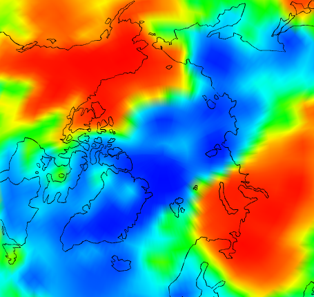
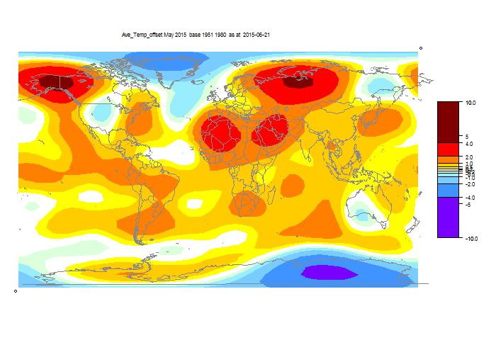
It's heavily weighted toward N and NE Siberia. I've added a facility, which I'll formalise, to the NCEP/NCAR map. The table on the right allows you to choose a day, by mousing over and tracking what it says just NE of the globe - click when you have what you want. It now allows you to choose the 0'th on the month, for Jan-May 2015, and you get the map of the monthly average anomaly. Selecting 2015-5-0, I get the May average map. Here's a plot of the Arctic region:
The reanalysis certainly shows cold anomaly in the Arctic, but nothing special in NE Siberia, and it was cold there in April too. That seems to be the main difference between GHCN and reanalysis.
Update. Here's another interesting table. This time I've weighted the anomaly differences to show their contribution to the TempLS sum. So when it says Qiqihar -0.00149, that means Q contributed that amount to the May-April anomaly difference. The weighted order is different to the absolute order, and the amounts are fairly small. The Antarctic now look more significant than the Siberian. The discrepancy between NCEP and GISS/TLS is of order 0.05°C, so none of these if changed would make more than 1/30 of that.
| May-Apr weighted | Latitude | Longitude | Name |
| -0.00174 | 51.12 | 99.67 | RINCHINLHUMBE |
| -0.00149 | 47.38 | 123.92 | QIQIHAR |
| -0.0013 | -68.58 | 77.97 | DAVIS |
| -0.00123 | 29.07 | -110.95 | HERMOSILLO,SO |
| -0.00123 | 79.5 | 76.98 | OSTROV VIZE |
| -0.00114 | -67.6 | 62.87 | MAWSON |
| -0.00105 | 67.25 | 167.97 | ILIRNEJ |
| -0.00102 | 45.97 | 128.73 | TONGHE |
| -0.00098 | 30.25 | 56.97 | KERMAN |
| -0.00093 | 53.7 | 91.7 | MINUSINSK |
Tuesday, June 16, 2015
GISS has global May temperatures same as April
GISS has reported an anomaly average of 0.71°C for May 2015, the same as for April. This is in agreement with TempLS mesh, but in contrast to the rise in the troposphere measures RSS and UAH.
I was surprised by the TempLS result, since the NCEP/NCAR index had indicated a much warmer result. HADSST3 also rose in May. But the GISS result essentially confirms it. It coincides with the new version 3.3 of GHCN, which would have influenced both indices. But that change made little difference to previous months. I am planning to post a study of the anomaly differences between April and May.
TempLS Grid also rose by about 0.05°C, so I think May rises in HADCRUT and NOAA are likely.
Below the fold is the customary comparison between GISS and TempLS.
Here is the GISS map for May:
And here is the corresponding TempLS map, using spherical harmonics:
Wednesday, June 10, 2015
TempLS May down slightly from April
GHCN Data was delayed slightly for May by the release of Version 3.3. When data became available, it was fairly complete. It showed a slight drop of 0.01°C from April (0.628 to 0.618). Satellite measures rose considerably.
Update 12 June. I'm still uncertain of this result. GHCN seems unsettled; according to my count, the most recent file has for May about 300 stations fewer than the day before.
This is at variance with the reanalysis data, which suggested a much warmer month. I wondered if V3.3 had an effect, but previous months were much as before. I'll watch the next few days for any changes, but as I said, most of the data is in. So May is looking more like April (cool for 2015) than February.
Details are in the report here. N Russia and Alaska had very warm spots; the poles were cool. The Arctic coolness was reflected in the reanalysis results. Generally the coolness was due to land; SST rose, as reflected by HADSST3.
There is an interesting Tech Note from NOAA on ver 3 here.
Thursday, June 4, 2015
Current Arctic Temperatures
I posted about a gadget for displaying NCEP/NCAR based average temperatures for user-selected Arctic regions. I have now embedded it in the maintained data page, so it will update whenever the other NCEP data does - usually daily. Operating guidance is at the original post.
Commenter Nightvid asked about including past years, and I'll do that sometime. It would overload the page to include the data by default, so I need a user-initiated download scheme.
I'm thinking of a similar gadget for whole Earth. The current one is for absolute temperatures, which is OK for special regions like Arctic. And it would be OK for, say, the NINO regions, but less good for continents, say. The alternative is anomalies, which don't show the seasonal effect. It's a dilemma.
Subscribe to:
Comments (Atom)


